Support Vector Machines for Automated Gait Classification - CiteSeerX

828

IEEE TRANSACTIONS ON BIOMEDICAL ENGINEERING, VOL. 52, NO. 5, MAY 2005

Support Vector Machines for Automated Gait Classification Rezaul K. Begg*, Member, IEEE, Marimuthu Palaniswami, Senior Member, IEEE, and Brendan Owen

Abstract—Ageing influences gait patterns causing constant threats to control of locomotor balance. Automated recognition of gait changes has many advantages including, early identification of at-risk gait and monitoring the progress of treatment outcomes. In this paper, we apply an artificial intelligence technique [support vector machines (SVM)] for the automatic recognition of young-old gait types from their respective gait-patterns. Minimum foot clearance (MFC) data of 30 young and 28 elderly participants were analyzed using a PEAK-2D motion analysis system during a 20-min continuous walk on a treadmill at self-selected walking speed. Gait features extracted from individual MFC histogram-plot and Poincaré-plot images were used to train the SVM. Cross-validation test results indicate that the generalization performance of the SVM was on average 83.3% ( 2 9) to recognize young and elderly gait patterns, compared to a neural network’s accuracy of 75 0 5 0%. A “hill-climbing” feature selection algorithm demonstrated that a small subset (3–5) of gait features extracted from MFC plots could differentiate the gait patterns with 90% accuracy. Performance of the gait classifier was evaluated using areas under the receiver operating characteristic plots. Improved performance of the classifier was evident when trained with reduced number of selected good features and with radial basis function kernel. These results suggest that SVMs can function as an efficient gait classifier for recognition of young and elderly gait patterns, and has the potential for wider applications in gait identification for falls-risk minimization in the elderly. Index Terms—Feature selection, gait analysis, histogram, minimum foot clearance, Poincaré plot, support vector machines.

I. INTRODUCTION

O

VER the years many research projects have been undertaken documenting kinematic, kinetic and electromyographic gait characteristics in the elderly (cf. [1]–[3]). One of the aims is to identify gait variables that reflect gait degeneration due to ageing that might have closer linkage to the causes of falls. This would help to undertake appropriate measures to prevent falls. Like in many other developed countries, falls in older population has been identified as a major health issue $billion per annum in Australia, costing the community [4]. Among the various fall types, tripping and slipping during walking has been identified to account for % of all falls [5]. While some research in ageing gait has looked at time-distance variables (e.g., walking speed, stance/swing times, step length), e.g., [6], others have carried out in detail biomechanical analyses

Manuscript received October 9, 2003; revised September 26, 2004. Asterisk indicates corresponding author *R. K. Begg is with the Centre for Ageing, Rehabilitation, Exercise and Sport, Victoria University, City Flinders Campus, PO Box 14428, Melbourne City MC, Victoria 8001, Australia (e-mail: [email protected]). M. Palaniswami and B. Owen are with the Department of Electrical Engineering, The University of Melbourne, Parkville, Victoria 3010, Australia (e-mail: [email protected]). Digital Object Identifier 10.1109/TBME.2005.845241

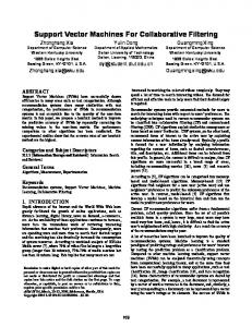
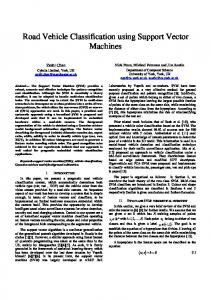
Fig. 1. Vertical displacement of toe marker for one gait cycle (foot contact to foot contact) showing the occurrence of MFC event during mid swing (toe-off to foot contact) phase.

to investigate differences between young and elderly populations; e.g., joint reaction forces, moments, powers [1]. It has been suggested that more sensitive gait variables such as foot clearance during walking over the walking surface should be used to describe age-related declines in gait in an effort to find predictors of falls risk [7]. Minimum foot clearance (MFC) during walking (see Fig. 1), which occurs during the mid-swing phase of the gait cycle, is defined as the minimum vertical distance between the lowest point under the front part of the shoe/foot and the ground, has been identified as an important gait parameter in the successful negotiation of the environment in which we walk. This is mainly because of the fact that during this MFC event, the foot travels very close to the walking surface (mean MFC cm) with a maximum forward velocity (4.6 m/s) [1]. The literature also suggests a decrease in MFC height ( cm) with ageing [1]. This small mean MFC value combined with the variability in MFC data ( – cm) has the potential to cause tripping during walking, especially for unseen obstacles or obstructions, thereby providing a strong rationale for MFC being associated with tripping during walking, and implication for trip-related falls in older population. Early identification of at-risk gait in older population provides the opportunity to undertake measures to prevent falls. At present, research in the area of automatic identification of gait types from their gait features is less prevalent. Neural network (NN) technology has been employed to classify various gait types. For instance, Barton and Lees [8] applied NN to differentiate simulated gait (e.g., leg length discrepancy) using features from lower-limb joint-anglemeasures, while Holzreiter and Kohle [9] applied NNs for classification of normal and pathological gait using force platform recordings of foot-ground reaction forces. Recently, supportvectormachines(SVMs),amachinelearningtechnique,have been shown to be a powerful tool for learning from data and for solving classification and regression problems with superior classification performance [10]–[14].

0018-9294/$20.00 © 2005 IEEE

BEGG et al.: SUPPORT VECTOR MACHINES FOR AUTOMATED GAIT CLASSIFICATION

829

to the constructed line in the transformed space are called the support vectors (Fig. 2) that contain valuable information regarding the OSH. SVM is an approximate implementation of the method of “structural risk minimization” aiming to attain low probability of generalization error [18]. Briefly, the theory of SVM is as follows [10], [17]. B. Basic SVM Theory The problem of pattern recognition may be stated as follows: Given a training data set , with input features and classification output, of the form

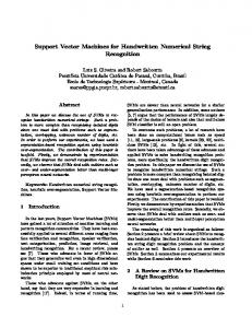
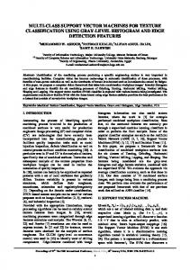
Fig. 2. An example of two-class (+ & o) problem showing optimal separating hyperplane (dotted line) that SVM uses to divide two groups’ data, and the associated Support Vectors. Data shown by ‘cross’ and ‘circle’ represent binary class +1 and 1, respectively.

0

In this paper, we propose to apply SVM technique for automated recognition of gait pattern changes due to ageing. As MFC heights are more likely to be associated with tripping during walking [7], [15] and these values tend to decrease with ageing [1], features derived from MFC distributions and plots were used to develop young-old classification models. This type of classification capability could potentially lead to many future SVM applications particularly as gait diagnostics: For example, SVM can be trained in a similar way to detect elderly fallers from their gait characteristics so that necessary measures can be undertaken to prevent injurious falls. The selection of SVM technology is primarily driven by the ability of the SVM to build improved predictive models. Unlike NNs, SVMs find an optimal separating hyperplane that provides superior generalization ability especially when the dimension of input data is high and the number of observations available for developing or training the model is limited [16]. Finally, classification results of the SVM classifier were compared with those obtained by a traditional NN with back propagation learning algorithm to compare their suitability as a gait classifier. II. SUPPORT VECTOR MACHINE (SVM) A. Overview of SVM SVMs are a relatively new machine learning tool and has emerged as a powerful technique for learning from data and in particular, for solving binary classification problems. SVMs originate from Vapnik’s statistical learning theory [10], and they formulate the learning problem as a quadratic optimization problem whose error surface is free of local minima and has global optimum [17]. In a binary classification task like the one in this study (young/old), the aim is to find an optimal separating hyperplane (OSH) between the two data sets. Fig. 2 illustrates a two-class problem with a hyperplane separating the two groups. SVM finds the OSH by maximizing the margin between the classes. The main concepts of SVM are to first transform input data into a higher dimensional space by means of a kernel function and then construct an OSH between the two classes in the transformed space. Those data vectors nearest

(1) for young gait and for elderly gait. We In our case, is is some unknown function to classify the feature assume vector (2) In SVM method, optimal margin classification for linearly separable patterns is achieved by finding a hyperplane in m dimensional space. The hyperplane must linearly separate the two on either side of the hyperplane. The equation classes of the decision surface (the hyperplane) is (3) where is the adjustable weight vector and b is the hyperplane bias. The linearly separable case can be represented mathematically as (4) Let is the optimal adjustable weight vector and is the optimal bias, where the optimal values are defined when the closest feature vectors are maximized (see Fig. 2). The optimization problem can be mapped to quadratic optimization problem with global minimum and linear constraints. The details of finding the values of and can be found in [17], [19]. In most real life problems (including our problem) the data are not linearly separable. One method is to apply nonlinear transforms to the original data, for example, creating a higher dimensional vector by multiplying all the terms in the feature vector with each other. While this may be manageable for small values of m, it quickly gets out of hand for larger values of m. This leads to the kernel trick that involves implicitly mapping our data from input space into a (usually much higher dimensional) feature space via a nonlinear kernel function, hiding the potentially high dimensionality of that feature space and, thus avoiding the curse of dimensionality [18]. The kernel function is related to the nonlinear feature mapping function by

(5) The fitness of a hyperplane in feature space is usually measured by the distance between the hyperplane and those training points

830


lying closest to it (the support vectors). A consequence of this is that we can completely specify our decision surface in terms of these support vectors. What initially hindered the widespread uptake of this early work was the inability to deal with nonseparable data in a satisfactory fashion. Two years after [20], Cortes and Vapnik put out a paper [19] that showed how a soft margin approach based could be used to tackle this problem in on slack variables a simple yet effective manner. The primal form of the problem given in this paper may be written

(6) is known as the regularization parameter. To avoid the curse of dimensionality, we do not attempt to solve the primal. Instead, we consider the Wolfe dual, namely

Also in [21], Schölkopf et al. mention the surprising experimental fact that any SVM, regardless of what kernel function is used, will tend to extract much the same set of support vectors. This result is important because it implies that we can radically vary the form of the kernel function using much the same incremental method as was used for variation. An overview of SVM pattern recognition techniques may be found in [23].

III. EXPERIMENTS To explore the SVM model and its application for binary gait classification task, we consider gait datasets involving young and elderly subjects. Particularly, MFC distribution features recorded during continuous walking were used to develop the SVM models as well as for testing classification performance of the models. In the following, we give a brief description of MFC data collection and feature extraction techniques, followed by performance evaluation measures for the models. A. MFC Gait Data

(7) where the variable is used to tune the tradeoff between minimizing empirical risk (ie. training errors) and the complexity of the machine. It turns out [21] that there is a strong link between SVM methods and the theory of structural risk minimization. In [21], Schölkopf et al. introduce the concept of the Vapnik-Chervonenkis (VC) dimension of a SVM, and prove that the cost minimizafunction is a tradeoff between empirical risk tion and minimization of the VC dimension. Based on this, we can state the pivotal risk bound result for SVMs. For a given SVM, there is a probability of that the following bound will hold:

(8) Further properties (including a number of tighter and more specialized theoretical performance bounds) can be found in [20], and [22].

MFC data of 58 healthy adults (30 young and 28 elderly) were taken from the gait database of the Biomechanics Unit of Victoria University. The young adults were from the academic community of Victoria University and the elderly participants were volunteers from various local senior citizen clubs. All subjects undertook informed-consent procedures as approved by the Victoria University Human Research Ethics Committee. The subjects had no known injuries or abnormalities that would affect their gait. Means and standard deviations (in brackets) of subject characteristics were as follows; Age (yr)—young 28.4(6.4), elderly 69.2(5.1); Height (cm)—young 171 (12), elderly 165(8); Body Mass (kg)—young 71.2 (15.0), elderly 66.9(8.3). Foot clearance (FC) data were collected during steady state self-selected walking on a treadmill using the PEAK MOTUS 2D (Peak Technologies Inc, Centennial, CO) motion analysis system. A 50 Hz Panasonic F15 video camera, with a shutter s, was positioned 9 m from the treadmill, perspeed of pendicular to the plane of foot motion to record unobstructed treadmill walking. Two reflective markers were attached to each subject’s left shoe at the fifth metatarsal head (MH) and the great toe (TM). Each subject completed about 20 minutes of normal walking at a self-selected comfortable walking speed. The MH and TM markers were automatically digitized for the entire walking task and raw data was digitally filtered using optimal cutoff frequency, which used a Butterworth filter with cutoff frequencies ranging from 4 to 8 Hz. The two-dimensional (2-D) motion measurement space was calibrated using a 1 m scaling rod with calibration markers attached to both ends. These markers were digitizedand their coordinates were used by the PEAK system to calculate a scaling factor, which was subsequently used for conversion of marker pixel coordinates to real distance units. The marker positions and shoe dimensions were used to predict the position of the shoe/foot end-point i.e., the position on the shoe travelling closest to the ground at the time when minimum foot clearance (MFC) occurs using a 2-D geometric model of the foot [15]. MFC was calculated by subtracting ground reference from the minimum vertical coordinate in the swing phase (see Fig. 1).


Q + MFC ) 2

831

Q

Q

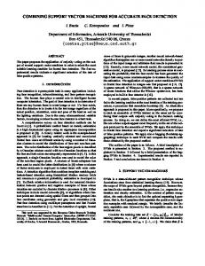
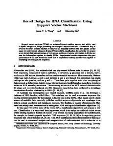
Fig. 3. (a) MFC histogram showing the main features extracted: —25th percentile, —median or 50th percentile, —75th percentile, Min—Minimum MFC, Max—Maximum MFC. Feature numbers and their descriptions are shown in the table. (b) MFC Poincaré plot showing the key features (in table) extracted from the plot along the major (Mean, = ) and minor (Difference, ) axes.

MFC = (MFC

B. Gait Feature Extraction Using MFC Histograms Each subject’s MFC data was plotted as histograms showing individual MFC data and their respective frequencies. Features describing major statistical characteristics of these distributions were extracted as illustrated in Fig. 3(a) and also shown in the insert. C. Feature Extraction Using MFC Poincaré Plots While MFC histogram plots show valuable statistical characteristics of the distribution, MFC plots of successive gait cycles, i.e., between and illustrate unique interaction effects in 2-D. Such plots, known as Poincaré Plots, have been shown to be highly effective in studying repetitive events, e.g., in heart rate variability research indicating relationships of R-R intervals to identify sound and abnormal heart function [24], [25]. Likewise, in analysing continuous gait function, these plots show unique relationship of MFC events between successive gait cycles and performance of the locomotor system in controlling the foot clearance at this critical event. For example, a low correlation in MFC Poincaré plots data would demonstrate less control since one stride is not affected by the previous stride [26]. Features characterizing these plots were used to develop young/old gait classification models. In the following, we show mathematical basis of the features extracted from these plots.

1MFC = (MFC

0 MFC )

Fig. 3(b) shows a typical MFC Poincaré plot. Variability of data along two perpendicular axes, represented by mean and difference are measures of short- and long-term variability in MFC data [25]. and Fromourimperialresultsitwasfoundthat are not statistically independent. Also a large number of MFC data points are measured so for practical purposes and . This leads to the following correlation matrix (9) where v is the variance of and c is the covariance of and . Given the data we require a transform so the resultant data is statistically independent (10) There are many transforms which produce two statistically independent measures, but we will look at the mean

832

and difference of fore, This leads to a transform


, there.

three segments. In this experiment, three types of kernel functions [17], [18], [28] were tested. 1) Linear 2) Polynomial (Poly) of degree “d”:

(11) The covariance of can be shown to be statistically independent (i.e., diagonal covariance matrix)

3) Radial Basis Function (RBF) with width “g”: (Appendix A) F. Neural Networks Gait classification between young and older adults was also carried out using neural networks (NNs) in Matlab. In this experiment, we used a three-layer NN with weights adjusted using thye Scaled Conjugate Gradient Algorithm [29] to train relationship between gait features and the respective gait class. The NN model had an input layer consisting of 24 neurons corresponding to the input gait features, one hidden layer and an output layer with two neurons representing gait types . After training a NN model, its generalization ability was evaluated using the three cross-validation test samples. G. Performance Testing Using ROC Plots

(12)

D. Cross-Validation Cross-validation is a standard test commonly used to test the ability of the classification system using various combinations of the testing and training data sets [8], [27]. In this method, performance of gait-class prediction is measured by systematically excluding some gait data during the training process and testing the trained model using the excluded gait trials. This process is repeated until every gait trial of the dataset is included in the testing data set. As the number of MFC data available was limited in this experiment (currently it takes about 60 h of digitization time with Peak Motus system to analyze one subject’s data), a 3-fold cross-validation test was applied in which 58 subjects’ data were divided into three segments with the testing data set (20) selected as: Segment 1 (1–20), Segment 2 (21–40), Segment 3 (38–58). Each of the three cross-validation test segments, therefore, had 10 young and 10 elderly subjects’ MFC data whereas their respective training segment included the remaining 20 young and 18 elderly subjects’ data. E. SVM Classifier All the gait features were normalized using their z-scores to have zero mean and unity variance prior to using them for training and testing the SVM. Software routines were developed in Matlab 6.0 (The MathWorks, Natick, MA) using SVM-Light1 for analyzing the gait data and to perform various tests, including tests to examine effects of kernel function, number of gait features and regularization parameter (C) on classification performance. The generalization performance of the trained SVM was determined by taking an average of the prediction accuracies and ROC areas (see Section III-G) of the 1http://ais.gmd.de/~thorsten/svm_light/

In addition to %classification accuracy, performance of the SVM classifier was tested using ROC (receiver operating characteristic) plots [14], [30]. The ROC curve displays plots of true positive rates or sensitivity (i.e., positively labeled test data classified as positive) versus false positive rates (i.e., negatively labeled test data classified as positive) as the threshold level of . False positive rates also classification is varied from 0 to . indicate specificity The area under the ROC curve provides a measure of overall performance of the classifier i.e., larger the ROC area the better is the classification accuracy over a range of thresholds. Many studies (cf. [14]) have used ROC plot and its area as an index for evaluating classifier performance. ROC curves were plotted for all SVM-kernels for different thresholds. Area under the ROC curve was computed numerically using custom made software routines written in Matlab. H. Hill-Climbing Feature Selection Generalization performance of a classifier depends primarily, among other factors, on the successes of selection of good features i.e., features that represent maximal separation between the classes [31]. A hill-climbing feature selection algorithm was used to identify features that provided the most contribution in separating the two classes across the three segments. This algorithm iteratively searches for features that positively improves or results in least reduction in separation results classification results. The search procedure may be described as follows. Let be the ROC area using a set of features, and let us start with two features sets: 1) Fixed features set, (initially empty); 2) Remaining features set, (initially all the features). Then, the fixed features set is incremented such that

where feature is chosen to maximize . This technique is repeated until all the features have been added to the fixed features set in descending order of their importance.


833

Fig. 4. Example (a) MFC histogram plots of one young and one elderly subject, and their respective (b) Poincaré plots. TABLE I ACCURACY OF PREDICTION (%) OF CROSS-VALIDATION TESTS USING LINEAR, POLYNOMIAL (d = 3) AND RADIAL BASIS FUNCTION (RBF) KERNELS AND NEURAL NETWORK USING ALL 24 FEATURES

IV. RESULTS Fig. 4(a) is an example of MFC distribution of a young and an elderly subject, whereas Fig. 4(b) shows their corresponding Poincaré Plots. These plots reveal some obvious qualitative differences between these two subjects, such as increased variability, lower MFC central tendency, and higher skewness (skewed to the right) in the elderly plots. Features extracted from these plots were used to train both linear and nonlinear SVMs as well as the NN, and later on test their capability to discriminate the two age groups. Table I shows mean success rates of the SVM classifier for the three cross-validation tests, which included all of the 58 subjects’ gait data in the test sample. The average success rate was % with a maximum accuracy of 85% in discriminating the gait patterns obtained with Linear and RBF kernels, and while trained with all 24 features. Tests with Polynomial (Poly) kernel provided lower accuracy, whereas when compared with the NNs results these results proved to be superior. Fig. 5(a), (b) displays ROC plots of Linear, Poly , and RBF kernels when all the 24 fea-

tures were used as inputs to the SVM classifier and also when only selected features were used to train the classifiers. With all 24 features, both Linear and RBF kernels showed better performance compared to the Poly kernel . However, when the classifiers were trained with selected features, their classification performance improved . This is also reflected in the shape of the ROC plots, i.e., higher sensitivities in RBF at higher specificities compared to the Poly kernel. Fig. 6 presents ROC areas plotted as a function of features selected by the (hill-climbing) feature selection algorithm. RBF displayed overall better performance relative to Linear and Poly kernels. It is important to note from these graphs that all three kernels attained their maximum performance with only a handful of features (3–5). The important features selected by the algorithm to achieve maximum ROC area include (see Figs. 3 and 6): Linear kernel—feature #13 (MFC coefficient of variation, CV), #20 and #4 (Q1); Poly kernel—feature #13 (CV), #16

834


Fig. 5. ROC (receiver operating characteristics) curves showing True positive (sensitivity) and False positive rates (1—specificity) for various thresholds using Linear, Polynomial (d = 3), and RBF (g = 1) kernels: (a) using all 24 features, (b) using selected features (3 for linear and polynomial, and 5 for RBF kernels) by the feature selection algorithm, C = 1. See text and Fig. 6 for details on feature selection.

TABLE II ROC AREA OF LINEAR, POLYNOMIAL (POLY) AND RADIAL BASIS FUNCTION (RBF) KERNELS FOR DIFFERENT REGULARIZATION PARAMETER (C) AND NUMBER OF FEATURES, d = DEGREE OF POLYNOMIAL, g = WIDTH OF RBF NETWORK

Fig. 6. Graph displaying the relationship between ROC area and the number of features selected by the “hill-climbing” algorithm for linear, polynomial (degree = 3) and RBF (g = 1) classifiers.

and #1

; RBF kernel—feature #13 (CV), #20 , #5 (Q2), #1 . Once maximum was achieved it was found to be fairly unaffected by further increment of gait features—eventually the graph showed a downward trend indicating that too many features negatively affected the classification performance. of the SVM classiTable II displays performance fiers as a function of number of gait features and also for three C values (.1, 1, 10). Overall, it emphasizes that all classifiers were able to discriminate well when trained with a fewer number of good features. Within the three classifiers, RBF kernel showed with and maximum performance . Fig. 7(a)–(c) shows scatter plots of the test data (Segment 3 results) with the separating hyperplane (decision surface) superimposed on the test data for the case of 1) Linear, 2) Poly, and 3) RBF kernels. These plots offer a visual representation of the two groups’ data as a function of first two features selected by the “hill-climbing” algorithm (feature #13 and 16). Examples of misclassification cases can be seen in all three kernels with individual test data being located on the wrong side of the separating hyperplane. Fig. 7(d) illustrates how a change in threshold , #18

level can affect the decision surface in a Poly kernel and, consequently its influence on classification accuracy. From Table II, it is also evident that the regularization parameter (C) can affect of the performance of the classifier. In Fig. 8, we plot linear kernel as a function of C using three subsets (3, 12, 24) of features selected by the “hill-climbing” algorithm. It is obvious from this plot that for the classifier, there is a range of C values that would yield optimum performance (e.g., with 12 features C would range between 0.8 to 8.6). Also, in this case the first 3-ranked features were found to provide the best classification results compared to those due to 12 and 24 features. From Figs. 6 and 8 we can see that there are both good and bad features in our data in terms of their contribution toward separating the two age groups. In Table III, we list the first 10 highly ranked features and their corresponding ROC areas in descending order. Histogram plot in Fig. 9(a) shows frequency of various combinations of 3 features and their corresponding


835

1MFC

Fig. 7. Two-dimensional scatter-plots showing test data and decision boundaries using two features (feature #13 (CV) and 16 (STD ) and 16) for the case of: (a) Linear, (b) Polynomial, and (c) RBF kernels (Segment 3 test results). (d) Diagram illustrating the effect of threshold change on decision boundaries and hence, classification performance for the case of a Polynomial classifier.

Fig. 8. ROC-area plots as a function of regularization parameter (C) for 3 different subsets of features (3, 12, and 24) using Linear kernel.

ROC areas, and confirms that there are features whose combinations would provide classification results of only by chance whereas other combinations can achieve a high . Fig. 9(b) illustrates alternative histogram plot using % classification accuracies, and reinforces the previous finding that some combinations of 3 features can yield a maximum accuracy of 90%. Features extracted from the MFC histogram plots were found to appear in about 60% of these

highest accuracy counts, whereas Poincaré plot features were found to be among the rest of the 40% counts. Statistical tests (T-tests) on the features of the MFC histogram plots revealed that nine out of the 13 features were significantly different between the two age groups. It is interesting to note that the best feature chosen by the SVM feature selection algorithm (feature #13, CV) was also found to be significantly different between the two age groups. Overall, features describing the central tendency of the distribution (i.e., mean, median) were % of the maximum acfound to be the main contributors curacy, whereas dispersion characteristics such as SD and InterQuartile-Range were responsible for nearly 30% of the con(11%) and higher tributions. Among other features, moment about short axis of Poincaré plots showed good contribution (12%) to the classification task. V. DISCUSSION In this paper, we propose a support vector machine based approach to classify young/old gait patterns. The results of this research suggest that histogram and Poincaré plots of MFC data provide useful information regarding the steady-state walking characteristics of individuals such that these features could be used to train a machine-learning tool to automatically recognize young/old gait. Early detection of locomotor impairments using

836


TABLE III TOP 10 RANKED FEATURES SELECTED BY THE ALGORITHM ACROSS THREE DATA SETS AND THEIR CORRESPONDING AVERAGE ROC

Fig. 9. Histogram plots showing the frequency of gait features (groups of three) and their classification outcomes: (a) ROC area, (b) % accuracy.

such supervised pattern recognition techniques would provide the opportunity to identify at-risk gait and initiate corrective measures to be undertaken, e.g., identify potential elderly fallers for falls prevention programs. Previous research on automated gait classification has used NNs and fuzzy clustering techniques for applications in diagnosis of pathological gait [9], [32]. Because of superior gait classification performance as demonstrated in this research and also classification in other biomedical applications [27], support vector machine appears to be a better alternative for automated gait diagnosis and also for such applications as monitoring the progress of treatment or intervention outcomes of gait in clinical and rehabilitation situations. SVMs are often time consuming to retrain, but using our technique of incremental learning [33] the retraining time can be reduced by orders of magnitude. In this study, MFC data from steady-state gait have been used to characterize gait patterns and as inputs to the SVM. There are two major reasons for this. Firstly, MFC provides a more sensitive measure of the motor function of the locomotor system compared to some gross overall kinematic descriptions of gait such as joint angular changes, and secondly, its close linkage with tripping risks [7], [15]. Tripping has been identified as a major cause of falls in older population. Also, MFC data collected over a longer duration are vital for the creation of histogram and Poincaré plots with sufficient data points so that their characteristics represent real gait performance. Insufficient

number of gait cycles due to data collected over short duration has the potential to result in distributions not reflective of individual’s gait performance. In fact to obtain a more stabilized gait pattern and to derive reliable statistics (e.g., mean, median, minmode, skewness, kurtosis etc.), MFC data recorded utes has been proposed [15]. All subjects in this study were fit and healthy and they completed the walking trial comfortably. When classification task of the SVM was compared across the three commonly used kernels: Linear, Radial Basis Function (RBF) and Polynomial, both the Linear and RBF kernels were found to perform well. The results of both SVM and NN classification tools suggest that the SVM-Linear and SVM-RBF performed superiorly when applied to separate young/old gait patterns. In a gender classification task using video sequence images, Lee & Grimson [12] also reported superior SVM performance with Linear kernel compared to a Polynomial kernel. Better classification performance by SVM over NN has been reported in another study involving protein fold recognition [27]. SVM eliminates many of the problems experienced with NN such as local minima and overfitting [17]. In addition, its ability to produce stable and reproducible results makes it a good candidate for solving many classification problems as evidenced by the recent surge in the use of this technique in many areas. Generalization performance of a classifier depends primarily, among other factors, on the successes of selection of good features i.e., features that represent maximal separation between the classes. A “hill-climbing” feature selection algorithm was employed here which iteratively searches for features that positively improves or reduces the least in identification results. The test results clearly show that with our gait data, only a handful of properly selected features (3–5) are necessary for effective classification. It is interesting to note that all three kernels picked as the best feature #13 feature in separating the two classes when “hill-climbing” algorithm was applied. This is not surprising as this is the only feature in our data set that contains information regarding the two most significant aspects of MFC distribution: variability and central tendency. The results displayed in Figs. 6 and 8 and Table II also reiterate that having many features would not be always helpful. In fact, when the maximum accuracy is obtained adding further features that are not good representative of the separation of two classes could have detrimental effect on the classification performance. Similar dependence of classification performance on features has been reported in other investigations. For example, in a movement classification task using features extracted from electroencephalographic signals, Yom-Tov and Inbar [34] demonstrated that only a small number of features (10–20) out of 1000 features were necessary to achieve maximum performance and the classification rate decreased for features . Similar conclusion has also been drawn using features taken from visual-field location measurements in Glaucoma diagnosis application using various machine classifiers [14].


837

shows clearly that useful gait features can be extracted using two types of MFC distributions—Histogram and Poincaré plots that can effectively separate young and ageing gait. Using results of this research we have demonstrated that SVMs are able to automatically recognize gait patterns of young and old, and appear to have plenty of potentials for future applications in identifying normal and pathological gait patterns. APPENDIX A Radial Basis Function (RBF)

Fig. 10.

One-dimensional Gaussian RBF with center x and width g .

Classification performance of the SVM also depends on the selection the regularization parameter, i.e., C as demonstrated in Fig. 8 and also in Table II. As we have already mentioned (Section II-B, (7)), C is the penalty parameter for misclassification and has to be carefully selected to achieve maximum classification accuracy. Fig. 8 also emphasizes that optimal value of C could be different for different number of features and has to be selected by trial and error method. One way of tackling this would be to plot a graph showing the reliance of classifier performance on C parameters and then picking the optimal C from the graph, similar to the one shown in Fig. 8. When compared across different C’s and number of features, RBF was found to perform the best in recognizing MFC gait-patterns , suggesting that RBF is able to better exploit the features compared to Linear and Polynomial classifiers. Both histogram and Poincaré plot features were effective in discriminating the two age groups. This suggests that gait changes with age are reflected in these plots and features extracted from these plots were instrumental in differentiating the two groups. Apart from MFC histogram features that provide statistical descriptors of MFC distributions, Poincaré plots have been extensively used in heart rate variability research for identifying normal/abnormal heart conditions from these plots [24], [25]. In our earlier work, Poincaré plots were used successfully in heart variability analysis [25] and for the first time, we have extended the analysis to gait, which has shown good promise in this area. It appears that such plots might also be useful in detecting movement abnormalities and also for monitoring improvements in walking performances as a result of treatment or intervention in a clinical/rehabilitation setting. Among the various features extracted from the two types of plots, features that are representative of MFC central tendency and variability measures were the main contributors of separation between the age groups. The research presented in this paper can be extended in several ways. In addition to kinematic gait features other gait characteristics such as force platform and electromyography results could be tried to investigate whether there are further improvements in its classification power. Furthermore, gait features associated with individuals with a history of falls could be used to train SVMs for automated identification of at-risk fallers. VI. CONCLUSION In this paper, we propose an automated gait classifier based on an emerging machine learning tool, support vector machine. It

The RBF [17], [18], [28] is a quickly and monotonically decreasing function as the data point x moves away from the center (see Fig. 10). The rate at which the Gaussian RBF decreases is governed by the width . The larger the value of g the slower is the rate of decline. Fig. 10 illustrates one-dimensional (1-D) RBF as a function of x. The 2-D RBF has similar cross section through its center, . Further details of RBF may be found in [17], [18], and [28]. ACKNOWLEDGMENT Several people contributed to the creation of gait database of the Biomechanics Unit of Victoria University. The authors wish to acknowledge all contributions especially, S. Taylor, L. Dell’Oro, and T. Karaharju-Huisman. This work was undertaken during outside studies program leave of Dr. R. Begg. REFERENCES [1] D. Winter, The Biomechanics and Motor Control of Human Gait: Normal, Elderly, and Pathological. Waterloo, ON, Canada: Univ. Waterloo Press, 1991. ˘ [2] J. O. Judge, R. B. Davis, and S. Ounpuu, “Step length reductions in advanced age: The role of ankle and hip kinetics,” J. Gerontol.: Med. Sci., vol. 51, pp. 303–312, 1996. [3] B. M. Nigg, V. Fisher, and J. L. Ronsky, “Gait characteristics as a function of age and gender,” Gait Posture, vol. 2, pp. 213–220, 1994. [4] B. Fildes, Injuries Among Older People: Falls at Home and Pedestrian Accidents. Melbourne, FL: Dove Publications, 1994. [5] T. M. Owings, M. J. Pavol, K. T. Foley, and M. D. Grabiner, “Exercise: Is it a solution to falls by older adults?,” J. Appl. Biomech., vol. 15, pp. 56–63, 1999. [6] K. M. Ostrosky, J. M. VanSwearingen, R. G. Burdett, and Z. Gee, “A comparison of gait characteristics in young and old subjects,” Phys. Ther., vol. 74, pp. 637–646, 1994. [7] M. G. Karst, A. P. Hageman, F. T. Jones, and S. H. Bunner, “Reliability of foot trajectory measures within and between testing sessions,” J. Gerontol.: Med. Sci., vol. 54, pp. 343–347, 1999. [8] J. G. Barton and A. Lees, “An application of neural networks for distinguishing gait patterns on the basis of hip-knee joint angle diagrams,” Gait Posture, vol. 5, pp. 28–33, 1997. [9] S. H. Holzreiter and M. E. Kohle, “Assessment of gait pattern using neural networks,” J. Biomech., vol. 26, pp. 645–651, 1993. [10] V. N. Vapnik, The Nature of Statistical Learning Theory. New York: Springer, 1995. [11] S. Ben-Yacoub, Y. Abdeljaoued, and E. Mayoraz, “Fusion of face and speech data for person identity verification,” IEEE Trans. Neural Netw., vol. 10, no. 5, pp. 1065–1074, Sep. 1999. [12] L. Lee and W. E. L. Grimson, “Gait analysis for recognition and classification,” in Proc. 5th Int. Conf. Automatic Face Gesture Recognition (FGR’02), 2002, pp. 1–8. [13] O. Chapelle, P. Haffner, and V. N. Vapnik, “Support vector machines for histogram-based classification,” IEEE Trans. Neural Netw., vol. 10, no. 5, pp. 1055–1064, Sep. 1999.

838

[14] K. Chan, T.-W. Lee, P. A. Sample, M. H. Goldbaum, R. N. Weinreb, and T. J. Sejnowski, “Comparison of machine learning and traditional classifiers in glaucoma diagnosis,” IEEE Trans. Biomed. Eng., vol. 49, no. 9, pp. 963–974, Sep. 2002. [15] R. J. Best, R. K. Begg, and L. Dell’Oro, “The probability of tripping during gait,” presented at the Int. Soc. Biomech. Conf., Calgary, AB, Canada, 1999. [16] N. Zavaljevski, F. J. Stevens, and J. Reifman, “Support vector machines with selective kernel scaling for protein classification and identification of key amino acid positions,” Bioinformatics, vol. 18, pp. 689–696, 2002. [17] V. Kecman, Learning and Soft Computing: Support Vector Machines, Neural Networks, and Fuzzy Logic Models. Cambridge, MA: MIT Press, 2002. [18] S. Haykin, Neural Networks: A Comprehensive Foundation. Upper Saddle River, NJ: Prentice-Hall, 1999. [19] C. Cortes and V. Vapnik, “Support vector networks,” Mach. Learn., vol. 20, pp. 273–297, 1995. [20] I. Guyon, B. Boser, and V. Vapnik, “Automatic capacity tuning of very large VC-dimension classifiers,” in Advances in Neural Information Processing Systems, S. J. Hanson, J. D. Cowan, and C. L. Giles, Eds. San Mateo, CA: Morgan Kaufmann, 1993, vol. 5, pp. 147–155. [21] B. Schölkopf, C. Burges, and V. Vapnik, “Extracting support data for a given task,” in Proceeding 1st International Conference on Knowledge Discovery Data Mining, U. M. Fayyad and R. Uthurusamy, Eds. Menlo Park, CA, 1995. [22] J. Shawe-Taylor, N. Cristianini, and , “Robust Bounds on the Generalization from the Margin Distribution,” Royal Holloway Coll., Univ. London, London, U.K., NeuroCOLT Tech. Rep. NC-TR-98-029, 1998. [23] C. J. C. Burges, “A tutorial on support vector machines for pattern recognition,” Knowledge Discovery Data Mining, vol. 2, no. 2, 1998. [24] P. W. Kamen and A. M. Tonkin, “Application of the Poincaré plot to heart rate variability: A new measure of functional status in heart failure,” Aust. NZ J. Med., vol. 25, pp. 18–26, 1995. [25] M. Brennan, M. Palaniswami, and P. W. Kamen, “Do existing measures of Poincare plot geometry reflect nonlinear features of heart rate variability?,” IEEE Trans. Biomed. Eng., vol. 48, no. 11, pp. 1342–1347, Nov. 2001. [26] S. Taylor, R. K. Begg, and R. J. Best, “An investigation of two methods for quantifying inter and intra-limb control/co-ordination processes of gait.,” in Proc. Int. Conf. Model. Simul., Melbourne, 2002, pp. 434–439. [27] C. H. Q. Ding and I. Dubchak, “Multi-class protein fold recognition using support vector machines and neural networks,” Bioinformatics, vol. 17, pp. 349–358, 2001. [28] C. Panchapakesan, M. Palaniswami, D. Ralph, and C. Manzie, “Effects of moving the centers in an RBF network,” IEEE Trans. Neural Netw., vol. 13, no. 6, pp. 1299–1307, Nov. 2002. [29] A. F. Moller, “A scaled conjugate gradient algorithm for fast supervised learning,” Neural Netw., vol. 6, pp. 525–533, 1993. [30] R. C. Sa and Y. Verbandt, “Automated breath detection on long-duration signals using feedforward backpropagation artificial neural networks,” IEEE Trans. Biomed. Eng., vol. 49, no. 10, pp. 1130–1141, Oct. 2002. [31] R. Begg and J. Kamruzzaman, “A machine learning approach for automated recognition of movement patterns using basic, kinetic and kinematic gait data,” J. Biomech., vol. 38, pp. 401–408, 2005. [32] M. J. O’Malley, M. F. Abel, D. L. Damiano, and C. L. Vaughan, “Fuzzy clustering of children with cerebral palsy based on temporal-distance gait parameters,” IEEE Trans. Rehab. Eng., vol. 5, no. 4, pp. 300–309, Dec. 1997. [33] A. Shilton, M. Palaniswami, D. Ralph, and A. C. Tsoi, “Incremental training in support vector machines,” in Proc. Int. Joint Conf. Neural Networks, Washington, DC, Jul. 2001. [34] E. Yom-Tov and G. F. Inbar, “Feature selection for the classification of movements from single movement-related potentials,” IEEE Trans. Neural Syst. Rehabil. Eng., vol. 10, no. 3, pp. 170–177, Sep. 2002.


Rezaul Begg (M’93) received the B.Sc. and M.Sc. Eng. degrees in electrical and electronic engineering from Bangladesh University of Engineering and Technology (BUET), Dhaka, Bangladesh, and the Ph.D. degree in biomedical engineering from the University of Aberdeen, Aberdeen, U.K. Currently, he is a Faculty member at Victoria University, Melbourne, Australia, where he researches in Biomedical Engineering and Biomechanics areas. His research interests focus on gait analysis, biomedical instrumentation, and artificial intelligence techniques. He has published over 80 articles in journals, conferences, and book chapters. He is currently involved in editing/co-editing two book volumes on computational intelligence techniques, and their applications in biomechanics and biomedical engineering areas, which are due to be published in 2005. He is a regular reviewer for several international journals. He chaired a number of conference sessions and was on the Technical Program Committee for several major international conferences. Dr. Begg has received several awards including the BUET Gold Medal and the Chancellor’s award for academic excellence.

M. Palaniswami (SM’95) received the B.E. (Hons.) degree from the University of Madras, Chennai, India, the M.E. degree from the Indian Institute of Science, Bangalore, India, the M.Eng.Sc. from the University of Melbourne, Parkville, VIC, Australia, and the Ph.D. degree from the University of Newcastle, Newcastle, Australia. He has been with the University of Melbourne for over 16 years. He has published more than 180 refereed papers with a majority of them in prestigious IEEE journals and conferences. His research interests include SVM’s, sensors and sensor networks, machine learning, neural network, pattern recognition, signal processing and control. He is the convener for Australian Research Network on Sensor Network. He is the Co-Director of Centre of Expertise on Networked Decision & Sensor Systems. Dr. Palaniswami received a Foreign Specialist Award from the Ministry of Education, Japan, in recognition of his contributions to the field of machine learning. He served as associate editor for Journals/transactions including IEEE TRANSACTIONS ON NEURAL NETWORKS and Computational Intelligence for Finance. He is the associate editor for the International Journal of Computational Intelligence and Applications and serves on the editorial board of the ANZ Journal on Intelligent Information Processing Systems. He is also the Subject Editor for the International Journal on Distributed Sensor Networks.

Brendan Owen received the Computer Science degree from the University of Melbourne, Parkville, VIC, Australia, in 1996, where he is working towards the Ph.D. degree. During 1996, he received the Electrical Engineering degree with honors from the University of Melbourne. He is currently a Senior Research Assistant and Tutor in the Department of Electrical and Electronic Engineering at the University of Melbourne. His interests include support vector machines, image processing, and computer vision.