Support Vector Machines for TCP Traffic Classification - CiteSeerX

Support Vector Machines for TCP Traffic Classification

Alice Este, Francesco Gringoli, Luca Salgarelli DEA, Universit` a degli Studi di Brescia,via Branze, 38, 25123 Brescia, Italy

Abstract Support Vector Machines (SVM) represent one of the most promising Machine Learning (ML) tools that can be applied to the problem of traffic classification in IP networks. In the case of SVMs, there are still open questions that need to be addressed before they can be generally applied to traffic classifiers. Having being designed essentially as techniques for binary classification, their generalization to multi-class problems is still under research. Furthermore, their performance is highly susceptible to the correct optimization of their working parameters. In this paper we describe an approach to traffic classification based on SVM. We apply one of the approaches to solving multi-class problems with SVMs to the task of statistical traffic classification, and describe a simple optimization algorithm that allows the classifier to perform correctly with as little training as a few hundred samples. The accuracy of the proposed classifier is then evaluated over three sets of traffic traces, coming from different topological points in the Internet. Although the results are relatively preliminary, they confirm that SVM-based classifiers can be very effective at discriminating traffic generated by different applications, even with reduced training set sizes. Key words: Traffic Classification, Machine Learning

1

Introduction

Traffic classification has recently become one of the hottest research topics in computer science and telecommunications for several reasons. The ability of assigning traffic flows to relevant classes of service is seen as a priority by many Internet Service Providers. Furthermore, the potential to detect the application behind a given IP flow is often at the basis of many security-related tools, such as anti-virus and anti-worm applications. Finally, algorithms for

Preprint submitted to Computer Networks

12 May 2009

traffic classification are essential for advanced network management and traffic engineering. The use of statistical approaches to Internet traffic classification has been the subject of quite a number of research efforts in the last few years. Much of the appeal of statistical or behavioral techniques for traffic classification resides in the hope that they will be able to work even in cases where port-based or payload inspection mechanisms fail. Examples where traditional classification techniques are increasingly loosing their effectiveness are in cases when explicit “anti-classifier” obfuscation techniques are employed by the end user applications, such as peer-to-peer or file sharing ones. Several recent papers have positively reported on the feasibility of machine learning (ML) approaches to traffic classification, relying exclusively on the statistical properties of the traffic to assign it to a specific service class, or even linking it to a particular application. Some of these techniques are particularly appealing because they seem to be able to discriminate traffic based on the analysis of only a few of the initial packets. They are therefore amenable to high-speed traffic classification, and they can be applied to the problem of assigning different Quality of Service (QoS) treatment to application flows on the fly. One of the most promising of such techniques is based on Support Vector Machines (SVM). Although some works on the application of SVMs to traffic classification are starting to appear, several points remain open as how to optimize their use to this specific machine learning problem. In this paper we tackle such open issues, and describe in depth an SVM-based traffic classifier that exhibits excellent performance while requiring minimal resources. The research contributions of this paper are the following: • We show the application of an SVM single-class approach for classifying the network traffic and for detecting outlier packets. Our classifier integrates the SVM “one-against-all” approach to solve multi-class problems when needed. • We introduce a simple optimization procedure to derive the ideal SVM parameters for the data sets we use, deriving a training procedure that operates on a limited set of elements. • We describe and analyze the results of the application of the SVM-based classifier to three data traces, two from large local area networks, and one from an Internet backbone. • We analyze the computational complexity of the classifier. The paper is organized as follows. In Section 2 we report on related work. Section 3 introduces the basic concepts behind Support Vector Machines. We describe in detail our approach to an SVM-based classifier in Section 4, while the following Section 5 reports on the experimental results we obtained by 2

running the classifier on three different data sets. Section 6 presents the analysis of some of the issues related to practical uses of our classifier, including a report on its computational complexity. Finally, Section 7 concludes the paper.

2

Related work

Since the pioneering studies by Paxson [1,2] on the statistical characterization of Internet traffic, lots of research has been done to develop classification systems using Machine Learning techniques, especially since the effectiveness of classical approaches based on port analysis and packet inspection has rapidly decreased. Several Machine Learning approaches to traffic classification have been developed and interesting results have already been published: these efforts have confirmed that the behavior of a traffic flow is so heavily influenced by the application that generates it that it is possible to detect the application protocol by simply observing a very limited set of features collected from the flow. Campos et al. [3] and McGregor et al. [4] show that traffic pattern similarity can be exploited to group observed flows into hierarchical clusters: they prove that different application layer protocols shape the generated traffic in such a way that the corresponding flows belong to the same cluster. They come to the conclusion that application protocols can be distinguished by classes - the clusters, i.e., bulk traffic, multimedia and so on - and they prove the effectiveness of unsupervised machine learning for coarse statistical traffic classification. A fine-grained classification based on clustering techniques is proposed by Bernaille et al. in [5]. In this work every flow is mapped to a n-dimensional space depending on features such as the size and the direction of its first n packets. Heuristics based on minimum distance criteria are used to assign analyzed flows to clusters. Roughan et al. [6] show that a useful set of features allowing discrimination between traffic classes can be located at different levels such as single packet, flow, connection and so on. They also show that a couple of ML based approaches - Nearest Neighbor and Linear Discriminant Analysis - can be used to classify network traffic. We have recently introduced a new supervised ML approach based on the notion of protocol fingerprints [7]. These objects provide a statistical behavioral description of the corresponding protocol: they take into account not only the size and the direction of the packets that compose a flow, but also interarrival times. They allow the classification of an unknown flow by measuring 3

“how far” it is from the relative descriptions. We showed with preliminary results how that algorithm is able to recognize with a very high degree of accuracy when a flow taken from a traffic aggregate belongs to one of the few fingerprinted protocols or not. In this work we put to use a different, less computationally–intensive technique based on SVMs, which does not rely on inter–arrival times. We also extend the experimental analysis to a larger set of protocols and a data set which is significantly more general. The usefulness of Support Vector Machines has been already demonstrated in several fields [8,9]: generally used for pattern recognition, SVMs, being not focused on local optimization, can provide optimal statistical classification by means of properly chosen decision functions. For example, they have recently been applied to identify and counter network DoS attacks showing very high accuracy [10,11]. Williams et al. [12] extensively reported about ML approaches for traffic classification. Although their contributions focus on several ML approaches, including Na¨ıve Bayes, C4.5, Bayesian Network and Na¨ıve Bayes Tree algorithms, they also consider SVMs in [13]. However, the SVM–based approach they describe seems to require a relatively complex tuning phase to achieve good results, which they decided anyway not to consider in their work. SVM for traffic classification also appears in a recent work by Li et al. [14]. The technique is used to train a classifier to recognize seven different classes of applications. The overall approach is quite different from ours since flows are divided in coarse classes such as bulk, multimedia, etc., while we consider a finer grained classification oriented to application detection. Nevertheless, the reported analysis is interesting as the authors point out how changing the features they consider influences the accuracy of classification results. To this end they propose an automatic algorithm for features selection and reduction from an initial human choice of nineteen elements. An additional difference of their work from ours is that we consider single quantities collected from packets as they are seen by the classifier – thus allowing almost real–time classification – while Li et al.’s algorithm can process a flow only after it is terminated.

3

Background on Support Vector Machines

Support Vector Machines represent a relatively new supervised learning technique suitable for solving classification problems with high dimensional feature space and small training set size. Although the basic technique was conceived for binary classification, several methods for single and multi-class problems have been developed. 4

Being a supervised method, it relies on two phases: during the training phase, the algorithm “acquires knowledge” about the classes by examining the training set that describes them. During the evaluation phase, a classification mechanism examines the evaluation set and associates its members to the classes that are available. During the training phase, the target of the algorithm is the estimation of boundaries between the classes described by the samples in the training sets. To describe the method with a very simple example one can think of a two class problem where a single regular surface perfectly divides the features space in two regions, each one fully representative of the corresponding class. Should this happen, then an exact boundary can be determined and no errors will be reported during the classification phase. Clearly this is not always possible and a trade off between the complexity of the boundary and the error rate must be chosen. Starting from the binary SVM technique [9], several extensions have been proposed to make SVMs suitable to deal with multi-class classification problems [15]. Although none of the multi-class approaches known in the literature is accepted as a solution to generic problems, SVMs techniques are nowadays mature enough to be applicable to many classification problems. In the following of this section, after a brief introduction on the main ideas behind two-class SVM, we describe the single-class approach and the multi–class technique we based our SVM traffic classifier on. This section is a brief introduction to the basics of SVMs, with the intent of clarifying how we applied the techniques to obtain our traffic classifier. As such, it is not meant to be an exhaustive introduction to the complex world of SVMs, and might be at times somewhat “compressed” in terms of presentation for obvious space constraints. Readers interested in a tutorial presentation of SVMs can refer, for example, to the work of Burges [16] or, for a specific introduction on ν-SVM, to the work of Sch¨olkopf et al. [17].

3.1

Binary (two class) SVM

Let us describe a generic classification problem, where a training set composed of m observations is available, each one belonging to one of two disjoint classes of elements. The i–th observation is identified by a feature vector xi ∈ Rn and a label yi ∈ {−1; +1} that indicates which class the observation belongs to. The aim of the SVM is to create a statistical model to predict the label value yi of an element considering only its attribute vector xi . Given the training samples, the SVM derives in Rn an optimal hyperplane that separates the two classes and that will then be used to assess the class 5

of unknown elements. The hyperplane equation is w · x + b = 0, where w is a coefficient vector, b is a scalar offset and the symbol “·” denotes the inner product in Rn , defined as:

w·x=

n X

(w)k (x)k ,

(3.1)

k=1

where (w)k and (x)k are the k–th scalar component of vectors w and x. The values of the optimal hyperplane parameters (w and b) are found maximizing the distance between the hyperplane and the nearest training observations of the two classes, that are called Support Vectors and that we will describe later in this section. Up to now we have seen only linear separation boundaries, that represent a too narrow class of functions. To perform a non–linear separation, the samples are mapped into another Euclidean space H through a non–linear mapping function Φ : Rn 7→ H. Within this space H, that has usually a higher dimension than original space, we determine the separating hyperplane w · Φ(x) + b = 0, that is a linear function of Φ(x) but corresponds to a non–linear boundary when is brought back in the Rn domain. If the inner product between two vectors Φ(xi ) and Φ(xj ) in H can be expressed as function of the corresponding xi and xj via a kernel function K : Rn x Rn 7→ R that satisfies the relation K(xi , xj ) = Φ(xi ) · Φ(xj ),

(3.2)

it is not necessary to explicitly specify the function Φ [16]. An example of K is the Gaussian kernel function, that we have chosen for the tests presented in this paper, defined as: 2

K(xi , xj ) = e−kxi −xj k

/2σ 2

,

(3.3)

where the norm kxi − xj k, that is equal to the square root of the inner product (xi − xj ) · (xi − xj ), represents the distance between the two samples xi and xj . We cannot know the explicit formulation of the mapping Φ, but from the Gaussian kernel expression we can deduce some information related to the location of vectors in H. We observe, firstly, that in H all the samples Φ(xi ) are located on a hypersphere centered in the origin of H and with radius 2 2 equal to 1, because kΦ(xi )k2 = e−kxi −xi k /2σ = 1 ∀i. Furthermore, when two vectors xi and xj are close in the initial space, the exponential in the equality 3.3 is close to 1, and remembering the geometrical interpretation of the inner product Φ(xi ) · Φ(xj ) = cos θ kΦ(xi )k kΦ(xj )k , where θ is the angle comprised 6

between Φ(xi ) and Φ(xj ), we can conclude that the two samples are close also in H. Otherwise, when the point xi is far from xj in Rn , the exponential is about 0; this implies that in H the vector Φ(xi ) is orthogonal to Φ(xj ). The Gaussian kernel is suitable for the data representation we adopt, presented in Section 4.1, where the class information is not linked to the position of vectors with respect to the disposition of the axes but only to the distance from the other samples of the same class. Within the space H the optimal hyperplane is determined from the training set samples {(xi , yi )}i=1,...m , imposing the maximum possible distance between the hyperplane and the closest points, by solving a quadratic programming problem with linear constraints. The Wolfe dual form of this problem is expressed with respect to variable α, a vector of m components αi , one for each training sample and it consists in the following minimization [18]:

min α

m X m 1X αi αj yi yj K(xi , xj ) 2 i=1 j=1

(3.4)

subject to

0 ≤ αi ≤ m X

1 m

αi yi = 0

i=1 m X

αi = ν.

i=1

This problem presents two free variables which ultimately affect the performance of the classifier: the Gaussian kernel width σ and the regularization coefficient ν. The former, that explicitly appears in the Expression 3.3, affects the disposition of vectors in H, while the latter parameter ν ∈ (0, 1] determines the fraction of training errors, i.e., the fraction of the training samples that fall in the wrong side of the hyperplane. We will describe the procedure we adopt for optimizing these parameters in Section 4.2. Once the solution α of the minimization problem 3.4 is found, the hyperplane parameter w is:

w=

m X

αi yi Φ (xi ) .

i=1

7

(3.5)

We can then express the decision function used by the classifier to establish the class of an unknown sample x as

f (x) = sign (w · Φ(x) + b) = = sign

m X

(3.6) !

αi yi K(x, xi ) + b .

(3.7)

i=1

This function evaluates on which side of the hyperplane the point Φ(x) lies, and returns the corresponding class label y. The offset value b can be determined considering two training samples xi with 0 < αi < m1 , that we call xN and xP of the class yN = −1 and yP = +1 respectively: 



m X X 1 b=−  αi yi K(z, xi ) . 2 z={xP ,xN } i=1

(3.8)

From the formulation of the decision function we observe that the classifier consists of an expansion of the training patters and only a subset of these defines the decision boundary. This subset is composed by the samples xi , called Support Vectors (SV), corresponding to αi > 0, because the remaining elements do not contribute to the sum in 3.6. Hence, the classifier complexity in the evaluation phase depends only on the number of the SVs. We will return to this concept later on when we will analyze the computational complexity of our classifier. 3.2

Single–class SVM

A single–class learning technique creates a model featuring a single class and it can be used when only one class of training samples is available. Although SVMs were originally designed for binary classifiers, Sch¨olkopf et al. in [19] proposed an approach to estimate, for a given class, the spatial region that contains most of the class patterns. The binary decision function, having the same form of Expression 3.6, is positive in the region holding the majority of the training vectors and negative outside the bound, where the patterns have dissimilar features compared to the samples of the training class. The edge of the region calculated with a single–class SVM has a non–linear shape in Rn (see Figures 3 and 4 for a few examples). The intuitive idea behind the one–class technique is to estimate in H the optimal hyperplane separating the mapped class vectors from the origin of the axes with the maximum possible margin. The second class, identified with label y = −1, is 8

thus composed of only one sample placed in the origin of H. In the case of Gaussian kernel, in the initial space Rn there does not exist a sample xi whose image is the origin of H, because, as we saw in the previous section, all vectors Φ(xi ) have unitary norm and lie on a hypersphere with radius 1. However, the mapped vectors Φ(xi ) appear in the Wolfe dual formulation of the problem only in the form of inner product K(xi , xj ) = Φ(xi ) · Φ(xj ). Therefore, when at least one of the two vectors is the origin 0 of H, the inner product Φ(xi ) · 0 =

X

(Φ(xi ))k 0

(3.9)

k

equals to zero, and it does not contribute to the sum in Equation 3.4 and in the decision Function 3.6. The single–class SVM model can finally be derived by removing from the sums the corresponding addends and combining the last two linear constrains in Equation 3.4 to remove also the corresponding αi . In the single–class case, due to the fact that only one element is present in the second class, optimizing the parameters of the classifier, such as the Gaussian kernel width σ and the regularization parameter ν, becomes even more critical than in the binary SVM case. We will describe our optimization procedures in Section 4.2. 3.3

Multi–class SVM

Several approaches have been developed to solve multi–class problems through binary SVM techniques. The simplest of them, that we adopt in this paper, is the one-against-all approach [15]. In an M –class classification context this method processes M binary problems: each one separates one class from the remaining (M − 1) ones. By training the corresponding M SVM models the following decision functions can be obtained:

w1 · Φ(x) + b1 w2 · Φ(x) + b2 ... wM · Φ(x) + bM .

(3.10)

As with the base binary SVM, the configuration parameters of the model, σi and νi , need to be optimized. Our simple procedure will be described in Section 4.2. 9

Finally, in the evaluation phase, a sample x is assigned to the class with the largest value of the decision function:

arg max {wi · Φ(x) + bi } . i=1,...M

4

4.1

(3.11)

A new SVM-based traffic classifier

Flow representation

In this paper we pursue the objective of recognizing the application-protocol responsible for sending packets through a monitoring node. After analyzing a few packets of each TCP flow, the monitoring node’s purpose is to assign the flow to one of the application classes it has been trained with, or to the unknown protocol class. We restrict the analysis to TCP traffic: the algorithm is set up to classify a flow that we define as the bi–directional ordered sequence of packets that are exchanged between a pair of connected endpoints, each one identified by an IP address and a TCP port. A flow is composed by packets as they are seen by the network device that collects them, possibly the node which hosts the classifier. Since we do not perform de–fragmentation or re–ordering, packets could be duplicated and out of order. We define as “semantically valid” a flow that begins with the TCP three–way–handshake and terminates with a complete TCP shutdown or when a packet with the RST flag set is seen. Packets inside a flow that carry no application payload are ignored by the classifier, because they do not introduce any additional information useful for the classification process. In fact, TCP packets with zero application-level payload are sent only to exchange connection state information, for example to set up the connection, to acknowledge the reception of packets or to regularly check if the connection is up (TCP keep alive algorithm). Therefore their features give us little information on the specific application protocol carried by the connection. After being captured, each flow is mapped to an ordered sequence of feature values based on each packet’s length. In order to discriminate the direction of the packets, we add to each packet length a constant value z, and change the sign of the obtained number when the packet is traveling from the server to the client. The value of z has been chosen in order to space points located in different quadrants keeping in mind the actual domain of the original data. The analyzed packets, in fact, travel on 802.3 network segments where the maxi10

mum packet size is 1500 bytes: this means that, if we set z = 1000, we end up with feature values lying in the intervals [−2500, −1040) and (+1040, +2500] (40 bytes is the minimum size for IP and TCP headers). We also remove the variable fields in the TCP header, used to send Options, because we are interested only in the length of data sent by the application level, thus the headers introduce a fixed offset of 40 bytes. Experimental results show that further increasing z does not lead to better classification results. The resulting mapping is expressed by the following relations: if Pkti sent by client:

Si = +size (pkti ) + z

if Pkti sent by server: Si = −size (pkti ) − z . Each flow is then associated to vector x given by

x = (S1 , S2 , S3 , ..., Sn ) ,

(4.1)

where n is the dimension of the space where each flow is mapped, i.e., the number of packets considered. If a flow carries less than n packets, we pad all missing Si to zero. The feature vector x is then used by the classification algorithm to guess which application protocol has generated the corresponding flow choosing from a finite set of protocol classes. To this end the first step of the SVM we are describing is to calculate the optimal separating hyperplanes between the vectors that belong to different classes: the “similarity criterion” used by the classifier to discriminate between application classes is the distance between the vectors in Rn that represent the flows. Following the requirement of working on the fly, i.e., being able to assign a flow to an application class after having considered only a few packets, our SVM classifier emits a verdict after seeing the first n packets of each flow. For the same reasons (real-time operation), we do not consider other “global” flow variables, such as flow length or the overall number of bytes carried by a TCP connection. The rationale behind selecting packet size as the main feature for our classifier is that the payload size should mostly depend on the finite state machine that drives the application layer protocol, especially in the early steps of the exchange. For example, if we consider the authentication phase in a mail retrieval connection, the POP3 protocol usually requires the client to send a couple of commands carrying the username and the password: this means that the corresponding flows will be located in a specific position in Rn . 11

In preliminary studies we also considered the inter–arrival time between consecutive packets as possible candidate for being included in the representative feature set. However, we found out that these quantities are less discriminating than Si for application identification and furthermore the noise due to network travel affects heavily their values. We will evaluate if it is possible to extract some useful information from inter–arrival times in a future work. The classification of extremely short connections is out of the scope of the classifier described in this paper. The rationale behind this is that flows that terminate very quickly after the establishment of the TCP connection are not amenable to their classification by observing their first packets: by the time the classifier would emit a verdict, the flow will have terminated. Therefore, we do not include in our training and evaluation sets flows with less than four payload–carrying packets. We chose this packet number specifically after verifying that the vast majority of the traffic volume in the traces we examined is generated by applications on top of TCP connections that have at least four payload–carrying packets. In Table 1 we show the proportion of flows and bytes corresponding to traffic of flows transmitting at least four packets with payload bytes. We evaluated these percentages on the three traces (listed in the first column) we used in our experiments, that we will describe in details in Section 5.1. The portion of short flows is significant (up to 50%), but the bytes globally carried in these connections are always less than the 6% of all the bytes transmitted in TCP flows; and if we consider only the payload bytes, the percentage of bytes decreases until the 5%. data set

flows

bytes

payload bytes

UNIBS

53%

98%

99%

LBNL

68%

99%

99%

CAIDA 49% 94% 95% Table 1 Proportion of traffic flows (and bytes) that are composed of at least four packets with payload.

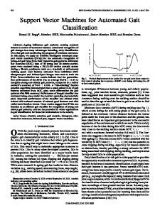
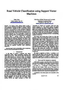
In Figure 1 we show an example of HTTP flows represented in the bi–dimensional space spanned by the first two components S1 and S2 : note that the HTTP flows are mostly distributed in the right part of the plane because the first message during a HTTP transaction contains a GET request sent by the client. If this request fits into a single TCP segment, the second packet will be sent by the server and we will get S1 > 0 and S2 < 0: in this case the corresponding points lie in the lower right part of the figure. If, instead, the GET request is larger in size, the first two packets are sent by the client: there could be a packet sent by the server in between but if present it should only carry an ACK flag without payload and therefore it is ignored by the classifier. In this second case both S1 and S2 are positive, and the corresponding packets lie in 12

Fig. 1. Vectorial representation flows for HTTP protocol (first two payload-carrying packets of each connection).

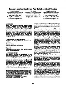
Fig. 2. Vectorial representation of flows for SMTP protocol (first two payload-carrying packets of each connection).

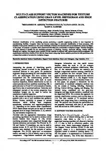
the upper right part of the figure. Figure 2 shows another example that depicts the features of SMTP flows. In this case the flows are distributed in a more concentrated region: in fact, the small area highlighted contains 99.47% of the flows. Port 25 is prevalently used to exchange e-mail messages through the SMTP protocol. According to the rules of SMTP the first packet carries a message sent by the server usually transmitting the 220 code meaning that the SMTP service is ready (S1 < 0), while the following packet comes from the client and it contains a HELO (or EHLO) message (S2 > 0). The remaining sparse 0.53% are mostly composed 13

of duplicated packets sent by the server, with S1 = S2 < 0. Although it is possible to represent the protocols in three or higher–dimensional spaces, their illustration on paper would not be that descriptive. However, in the rest of the paper we will consider multi–dimensional spaces.

4.2

4.2.1

Training phase

Ground truth

In this paper we refer with the term “class” to the set of flows generated by the same application–layer protocol. We partition the training set according to the result of a pre–classification stage separating the traffic flows in different protocol classes. To achieve an accurate model of each class, the flow vectors belonging to the training set need to be sufficiently representative of all the protocols the classifier is trained to identify. To this end, if application–layer payloads are available in a traffic data set, we use a payload–based pattern– matching technique to group flows, according to the patterns reported in [20]. When pattern–based pre–classification is not possible, for example because the available traces have been fully anonymized, we group traffic according to the server transport layer port. In the second case, obviously, we cannot ensure the accuracy of the training (and evaluation) sets: it can happen, in fact, that some flows use a given port just to bypass a policy restriction and they do not correspond to the expected application protocol. Although we wish that there were a more precise mechanism to assess the ground truth of each of the anonymized traces we used, it is clear that no mechanism other than port analysis is possible with fully anonymized traces such as the ones released by large organizations. At any rate, the use of ports as a substitute for ground truth is a practice accepted in the literature in these cases.

4.2.2

Single–class models

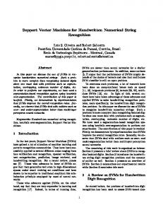
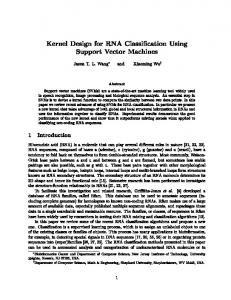
During the training phase the classifier optimizes its structure and parameter values. Our algorithm builds a single–class SVM model for each application class Ci by feeding the classifier with flows from each class of the training set. This step ends up with one separating surface for each protocol defined in an n–dimensional space: this surface contains the training observations with a confidence level determined by the parameter ν. In Figure 3 we show an example of the separating surface determined in a bi– dimensional space for the HTTP protocol. Changing ν causes modifications to the shape of the separating line, and this in turns modifies the number of 14

Fig. 3. Separating line corresponding to n = 2, σ = 300 and ν varying in {0.1, 0.07, 0.04, 0.01} for http traffic.

Fig. 4. Separating line corresponding to n = 2, σ = 14 and ν varying in {0.1, 0.07, 0.04, 0.01} for SMTP traffic.

observations that fall inside the line itself. In Figure 4 we show an analogous example of the single–class learning result for SMTP flows. The values of ν, σ and n are chosen through a grid search defined in the space of parameters to optimize the classification accuracy. We determine the 15

optimum value of parameters for the class Ci according to the percentage of vectors of the training set that are correctly classified as elements of Ci . In other words, the optimization criteria that we use to choose the configuration parameters is that the separating surface for each protocol should include as many elements of the corresponding class as possible. It is necessary to force the surface boundaries to not overly extend than the spatial region actually holding the class Ci vectors, so that flows generated by protocols other than the class under consideration are not included. To this end, we use the samples of the remaining M –1 training classes as outlier samples, to minimize the percentage of flows of other training classes that are incorrectly attributed to Ci . Furthermore, to guarantee that protocol classes not appearing in the training set are left out from class Ci ’s surface, we consider a further class Cu with a uniform distribution. This class samples are generated considering the variables Si independent and uniformly distributed between [−2500, +2500]. We choose this distribution model because we do not know any information related to the flow position and therefore we suppose that they can be in any space region with equal probability. Experimental results show that the introduction of the class Cu is useful to increase the accuracy of the classifier when dealing with protocols that occupy large regions. The parameter values for class Ci are chosen according to the following expression:

arg max { Hi (ν, σ, n) − Fi (ν, σ, n) } , (ν,σ,n)

where Hi is the percentage of training flows of class Ci that are correctly located inside the surface, while Fi is a combination of the percentages of other protocol flows locating in the surface of class Ci , defined as:

Fi (ν, σ, n) = γ ·

M X

1 · Fji (ν, σ, n) + (1 − γ) · Fui (ν, σ, n). j=1,j6=i M − 1

The symbol Fji denotes the percentage of training flows of the class Cj lying in the decision surface of Ci , while Fui is the percentage of vectors drawn from the uniform distribution located inside the surface. The coefficient γ, with 0 < γ < 1, establishes how each of the two addends of the expression 4.2 affects the decision surface of the class Ci . In the experiments described in this paper we choose γ = 21 so as to give the same weight both to the recognition of the correct class and to the detection of an outlier. Since this phase requires, for each tuple (ν, σ, n), the solution of the quadratic programming problem that we have seen in Section 3.2, it is fairly computa16

Fig. 5. Single-class classifier precision vs. number of flows selected from the training sets.

tional intensive. To reduce the complexity of the training phase, we found out that randomly selecting four hundred flows from the training set for each class seems enough to correctly train the classifier for each considered protocol. Figure 5 shows the maximum value assumed by the argument in Expression 4.2 varying the number of flows selected from the training set. The values seem stable enough when using 400 flows. The selection of a restricted number of training samples implies a further advantage: since the number of support vectors is limited because they are a subset of the input vectors, the complexity of the evaluation phase is greatly reduced.

4.2.3

Multi–class phase

Let us consider now the second stage of our classifier, that implements a multi– class SVM algorithm. To build the multi–class model we employ in all the M binary SVM the same set of parameters (ν, σ, n), to limit the complexity of optimizing them for each one-against-all case. We find the optimum set maximizing the following relation:

arg max

(ν,σ,n)

(M X

)

Hi (ν, σ, n)

,

i=1

where Hi is the percentage of training flows of class Ci correctly classified. To train the classifier for each one-against-all binary SVM we use two hundred samples randomly extracted from the training set of each protocol. The complementary class, representing all the remaining protocols, is composed by two hundred observations randomly extracted from their training set. 17

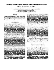
Fig. 6. Classification procedure.

4.3

Classification procedure

Once the relatively complex training phase is completed, our classifier works as shown in Figure 6. In order to classify an unknown flow “x”, the classifier finds what surfaces, among the ones calculated during the training phase, the corresponding feature values fall in: if there is only one candidate surface, then the flow is assigned to the corresponding class (i.e., application protocol). If, instead, the flow falls outside all the available surfaces, the flow is marked as not being generated by any of the known applications. In some cases it may happen that the flow falls inside the surfaces of two or more different classes. In this case, to assign the flow to a class, a further multi–class SVM stage is required, as explained above and in Section 3.3.

5

Experimental results

In this Section we present the numerical results obtained by classifying three different sets of traffic traces. The first was collected at the edge router of our Faculty network, and we indicate it as the UNIBS set. The other two sets are 18

derived from public anonymized traces from the Lawrence Berkeley’s National Laboratory (LBNL) and from the Cooperative Association for Internet Data Analysis (CAIDA) repositories. The first set is very useful because, even though it is not publicly available, the traces have been captured preserving the first 400 bytes of each packet. Therefore, it is relatively simple, by means of pattern–based methodologies, to ascertain the “ground truth” on which protocol generated which flow, at least for non-ciphered traffic. This makes it easier to generate correct training and evaluation sets. The traces from the other two sets have been payload–stripped and fully anonymized. Therefore, the only pre–classification methodology that can work to build training and evaluation sets from them is relying on port–based analysis, which can of course be less than precise. However, results from these two anonymized sets are important because prove the general applicability of our classifier.

5.1

5.1.1

Description of data sets

UNIBS data set

The packet traces from this set were collected at the border router of our Faculty network. Since we have full monitor access to this router, we captured the first 400 bytes of every packet. We can hence apply pattern-matching mechanisms to assess the actual application that has generated each TCP flow, in some cases with the addition of manual inspection. At any rate, because of this, we consider both the training and evaluation sets derived from UNIBS relatively reliable with respect to the pre-classification information, i.e., with respect to knowing, independently from our classifier, which application generated each flow. Our network infrastructure comprises several 1000Base-TX segments routed through a Linux-based dual-processor box and includes about a thousand workstations with different operating systems. All the traffic traces were gathered on the 100Mb/s link connecting the edge router to Internet during the first three weeks of June of 2007. A total of 50GB of traffic was collected by running Tcpdump [21] for fifteen minutes regularly every hour. Both the training and the evaluation sets are composed of protocol classes belonging to different application types: web browsing, mail services, P2P and interactive. They were chosen because they are responsible for the generation of the most part of the traffic, and because, given their variety, they allow us to verify the general applicability of our SVM–based technique. In addition, 19

they are easily identifiable with pattern-matching methods with a satisfactory degree of accuracy and precision. Though only four hundred vectors for each class were taken from the training set, we needed to collect many more flows: there is, in fact, a noticeable correlation between flows whose capture times are close – i.e., they are often generated by the same source. Since we need a complete description of the protocol features, we collected much larger traces and extracted only a small, random subset for the training phase. We inserted in the training set the first six protocols listed in Table 2. We report, next to each protocol name, the percentage of flows that it has generated and the portion of bytes that it has transmitted; in the last column we consider only the percentage of the bytes corresponding to the application–layer. protocol

flows

bytes

payload bytes

http

65.35%

79.55%

79.89%

smtp

5.92%

1.63%

1.54%

pop3

1.74%

0.25%

0.23%

ftp

0.13%

0.01%

0.003%

bittorrent

0.81%

1.78%

1.74%

msn

0.24%

0.04%

0.04%

edonkey

7.71%

3.22%

3.17%

ssl

6.55%

1.46%

1.41%

smb 0.05% 0.003% 0.002% Table 2 Composition of the traffic gathered at UNIBS border router.

In addition to the six protocols mentioned above, we included the other three classes of flows in the table in the evaluation set. These classes were used to verify the classifier’s ability to recognize protocols different than those used during the training phase. We took care of choosing the training and evaluation sets from traces collected in two different and consecutive time frames.

5.1.2

LBNL data set

The LBNL traffic traces were collected at the Lawrence Berkeley National Laboratory [22] and were anonymized using the tool tcpmkpub described in [23]. The packet traces were gathered at the two central routers of the LBNL network and they contain traffic generated from several thousand internal hosts. The measurement system allowed to store at the same time the traffic of only 20

two of the 20+ router ports. Hence, periodically, the corresponding monitored subnets changed and the resulting traces were originated from the succession of the subnets in turn. This measurement procedure impacts the characteristics of the LBNL traffic traces, since for each application protocol the number of flows and their statistical properties can depend on which subnets were monitored. For example, if at a given time the two monitored subnetworks include a large mail server, the corresponding trace will contain mostly e-mail traffic, and the flows will be generated by a restricted number of hosts [24]. We partly reduce these effects by randomly extracting from the whole training set the vectors used for the training phase, including traffic from all the available subnets. We used the traffic traces captured on December 15 and 16, 2004 to obtain the training set and those captured on January 6 and 7, 2005 to build the evaluation set. The selection of protocols is different with respect to the UNIBS experiment and it includes for the training phase the first six classes in Table 3. In the evaluation set we also consider the remaining eight classes we show in the table. port

expected protocol

flows

bytes

payload bytes

80

http

33.68%

41.88%

42.32%

25

smtp

6.21%

9.75%

9.92%

110

pop3

0.73%

0.20%

0.19%

443

https

7.89%

3.84%

3.84%

993

imaps

2.24%

3.64%

3.66%

139

netbios

2.28%

2.37%

2.31%

445

smb

2.15%

0.78%

0.72%

389

ldap

1.67%

0.25%

0.23%

5308

cfengine

0.62%

0.19%

0.09%

631

ipp

0.95%

0.09%

0.05%

21

ftp

0.23%

0.01%

0.01%

995

pop3s

0.57%

0.14%

0.13%

515

printer

0.10%

0.43%

0.44%

22

ssh

0.39%

7.35%

7.43%

Table 3 Composition of the traffic of the LBNL data set.

We excluded those protocols for which we did not have a sufficient number of flows to run the experiments. Since we need as many flows as possible to 21

characterize a given protocol, we analyzed the traces to determine the most common applications and we grouped them to form the compositions reported in the table. A positive side effect of this procedure is that the protocols we analyzed account for the vast majority of the traffic contained in the data set. We observe that in the LBNL data set there are not packets with TCP ports usually used by peer-to-peer services, such as 1214/kazaa or 6881/bittorrent, likely as a consequence of security policies that do not allow this kind of traffic.

5.1.3

CAIDA data set

The CAIDA data set contains anonymized traces collected during three hours at AMES Internet Exchange (AIX) along an OC48 link on August 14, 2002. We used flows extracted from the first hour (corresponding to the interval 16.15-17.00 UTC) to build the training set and from the third hour (18.0018.10 UTC) to create the evaluation set [25]. We used the CAIDA traces to verify the applicability of our classifier to backbone links, where high transmission rate are common and the traffic sources can be more heterogeneous than in local networks. The procedure we used to select the protocols is the same as the one followed for the LBNL data set. The flows used in the training set correspond to the first six classes we show in Table 4. We included the remaining five protocols in the evaluation set. port

expected protocol

flows

bytes

payload bytes

80

http

84.69%

81.58%

81.71%

25

smtp

4.57%

2.72%

2.47%

110

pop3

0.60%

0.25%

0.24%

21

ftp

3.32%

0.09%

0.03%

443

https

2.13%

0.90%

0.88%

4662

edonkey

0.79%

1.35%

1.34%

1214

kazaa

0.30%

3.28%

3.36%

6346

gnutella-svc

0.11%

0.20%

0.19%

119

nntp

0.03%

0.14%

0.15%

53

dns

0.01%

0.001%

0.001%

gnutella-rtr

0.01%

0.01%

0.01%

6347

Table 4 Composition of the traffic classes of the CAIDA data set.

22

5.2

Classification results http

smtp

pop3

ftp

bittor

msn

unknown

http

94.9%

–

–

–

–

–

5.1%

smtp

–

92.3%

0.1%

0.7%

–

–

6.8%

pop3

–

0.4%

88.2%

3.7%

–

–

7.7%

ftp

–

–

0.5%

97.7%

–

–

1.8%

bittor

1.8%

–

–

–

96.8%

–

1.4%

msn

–

–

–

–

0.1%

91.2%

8.5%

edonkey

–

–

–

–

–

–

100.0%

ssl

29.7%

–

–

–

–

–

70.3%

smb – – – – – – 100.0% Table 5 Classification results for the UNIBS data set. True Positives are in bold.

Classification results from the UNIBS data set that we show in Table 5 look very promising. Most of the applications for which the classifier was trained are recognized with True Positives above the 90% mark and with very low False Positive rates. The 88.2% of pop3 flows correctly classified is the only sub–standard result compared with the mean percentage of True Positives of the other application protocols and the 3.7% of pop3 traffic classified as belonging to ftp denotes that the classifier has some difficulties in discriminating between these two protocol classes. We observe that the pop3 and ftp protocols present a similar message exchange in the authentication stage, in which the client sends in both cases its username and password with ASCII strings introduced respectively by the keywords “USER” and “PASS”. Hence, the space regions that the two classes inhabit are very close and the optimum packet number n the classifier requires in the single–class phase to distinguish these protocols is greater than the other applications, especially for pop3 protocol, as we report in Table 6. Anyway, the statistics of the username length show some differences for pop3 and ftp traffic, because ftp often transports shorter standard username such as the “anonymous” string. The identification of flows representing outliers with reference to the training classes has a high accuracy level. The class we named ssl contains all the application protocols that work on top of TLS or SSL. These protocols are mostly represented by https, pop3s and imaps. Our classifier assigns to the http class a relatively high (29.7%) number of flows belonging to the ssl class. The majority of these mis-classified flows falls perfectly inside the surface of 23

single–class

multi–class

Nsv

n

Nsv

n

http

21

3

244

5

smtp

33

2

157

5

pop3

30

6

116

5

ftp

27

3

211

5

bittor

26

2

217

5

msn

26

3

176

5

Table 6 Support Vector number Nsv and space dimension n for each class of the UNIBS data set, as determined by the optimization procedure executed during the training phase.

the http protocol during the single–class classification phase, in fact ssl transmits immediately a large data quantity, especially when the server sends its certificate, therefore the ssl handshake packets assume similar feature values to the web request-response phase. 80

25

110

443

993

139

unknown

80

83.5%

–

–

–

–

–

16.5%

25

–

98.5%

–

–

–

–

1.5%

110

–

2.7%

95.7%

–

–

–

1.5%

443

6.6%

–

–

69.6%

0.2%

–

23.7%

993

1.0%

–

–

–

97.3%

–

1.7%

139

–

–

–

–

–

100.0%

–

445

–

–

–

–

–

–

100.0%

389

11.0%

–

–

0.7%

9.0%

–

79.3%

5308

–

–

–

–

–

–

100.0%

631

–

–

–

–

–

–

100.0%

21

–

0.6%

79.2%

–

–

–

20.1%

995

–

–

–

12.8%

74.7%

–

12.5%

515

–

–

–

–

–

–

100.0%

22 – – – – – – 100.0% Table 7 Classification results for the LBNL data set. True Positives are in bold.

The classification results achieved on the LBNL evaluation set are reported 24

in Table 7. The percentage of flows correctly classified lies between 69.6% and 100.0%, where the lowest results are obtained for the 443/https and 80/http ports. We observe in the table that the class marked by the 139/netbios-ssn port reaches the 100% of correct identification and no flows generated by other protocols fall in its specific region. These flows are, in fact, internal traffic produced by nodes inside the LAN and their statistical features are more regular and homogeneous than flows coming from external network. The relatively low figure for the True Positives of the 80/http class can be attributed mostly to the way the LBNL traces were collected. As explained in [24], web transactions recorded in this trace included activities that differ from traditional user-browsing, such as programs running on top of http (e.g Novell iFolder and Viacom NetMeeting) or Google bots [24]. These different activities assembled in a unique class (the one of the traffic directed to TCP port 80) and the difference in http traffic generated by different subnets cause some differences in the distribution of vectors between the training and evaluation sets. To obtain a more accurate description of this traffic it would be necessary to create different models for the several activities that use the same port 80/http, but that would require the traces not to be fully anonymized. The True Positives for 443/https are relatively low at just below the 70% mark. Examining this issue, we found out that the features of the 993/imaps protocol are quite similar to the ones of 443/https, making it harder for the classifier to discriminate flows produced by the latter protocol. This observation is supported by the higher than usual value for the n parameter (the length of the feature vector, as shown in Table 8) of 443/https as calculated by the optimization procedure, which confirms that the identification of the proper region for this protocol is more difficult than for the others. Even in this case outlier protocols are correctly recognized with a good confidence level. The only classes that present relatively high False Positive rates are the 21/ftp and the 995/pop3s. The 79.2% of the 21/ftp flows are classified as 110/pop3 and the 87.5% of the 995/pop3s flows are recognized as 443/https or as 993/imaps. We believe that discriminating these two protocols requires the design of a classifier that operates on more features that packet size alone. Results of the classification of the CAIDA evaluation set are reported in Table 9. They show a good accuracy for the protocols used in the training phase, while the classification of the outlier classes leads to less precise identification. The CAIDA data set contains traces that were recorded in a brief time interval: in fact the training and evaluation sets differ, temporally, at most by two hours. Therefore the flows captured for each port present similar statistical properties and the correct classification percentages of the six protocols are higher than 25

single–class

multi–class

Nsv

n

Nsv

n

80

42

3

293

3

25

12

4

212

3

110

22

3

228

3

443

52

5

44

3

993

8

4

319

3

139

40

2

331

3

Table 8 Support Vector number Nsv and space dimension n for each class of the LBNL data set, as determined by the optimization procedure executed during the training phase. 80

25

110

21

443

4662

unknown

80

94.7%

–

–

–

1.0%

–

4.3%

25

–

86.5%

3.6%

–

–

–

9.9%

110

–

0.5%

95.1%

0.1%

–

–

4.4%

21

–

0.5%

0.2%

97.9%

–

–

1.5%

443

0.1%

–

–

–

97.8%

–

2.2%

4662

–

–

–

–

–

98.8%

1.2%

1214

67.1%

–

–

–

15.5%

5.7%

11.7%

6346

64.1%

–

–

–

4.1%

2.4%

29.4%

119

–

58.3%

15.0%

–

–

–

26.7%

53

45.7%

–

–

–

25.7%

–

28.6%

6347 51.6% – – – – – 48.4% Table 9 Classification results for the CAIDA data set with the SVM–based classifier.

86.5%. However the recognition of the flows belonging to the outlier classes does not appear so accurate. We attribute this fact to the more various characteristics that the protocol features have in a backbone link compared to the traffic traveling in a LAN. Furthermore we observe, as we have seen for the UNIBS data set, that the peer-to-peer traffic of the 1214/kazaa, 6346/gnutella-svc and 6347/gnutella-rtr classes is attributed by our classifier to the 80/http class. Also kazaa relies on 26

http to transfer files. As we did for the other two data sets, we show in Table 10 the Support Vector number Nsv and the space dimension n our optimization procedure found for each class. single–class

multi–class

Nsv

n

Nsv

n

80

16

2

258

5

25

43

6

178

5

110

21

6

133

5

21

17

3

167

5

443

8

2

233

5

4662

9

2

159

5

Table 10 Support Vector number Nsv and space dimension n for each class of the CAIDA data set, as determined by the optimization procedure executed during the training phase.

6

6.1

Discussion

Computational complexity

In this section we evaluate the computational complexity of the SVM–based classifier. We limit our evaluation to the analysis of the actual classification phase, rather than the training one, because we want to point out what operations need to be completed in real time to identify the flows passing through a monitoring node, while the training phase can be performed off-line and thus its complexity is less critical. In the single–class stage, to estimate if a flow x falls inside one of the surfaces describing a training class in a n-dimensional space, it is necessary to compute the value of the decision Function 3.6, that is the sign of the following expression:

N sv X

2

αi e−kx−xi k

i=1

27

/2σ 2

+b ,

(6.1)

where Nsv denotes the number of the Support Vectors xi . To evaluate the complexity of the classifier according to the basic operation number that it is necessary to execute for each test element x, we consider the following set of steps that the classifier performs for each protocol class: 1: 2: 3: 4: 5: 6: 7: 8: 9: 10: 11: 12: 13: 14:

q=0 for i = 1 : Nsv r=0 for j = 1 : n w = x[j] − xsv [i][j] w =w·w r =r+w end r = −1/2σ 2 · r r = exp(r) r = α[i] · r q =q+r end q =q+b Fig. 7. Basic sequence of steps for the SVM single–class phase.

The computation complexity increases linearly with the number of the Support Vectors Nsv and the space dimension n. The sequence of steps that we show in Figure 7 is repeated for each of the M classes appearing in the training set, thus the overall algorithm has a linear dependency also from the number of training classes, i.e., the number of considered protocols. The order of magnitude of the computation complexity of the single–class stage is therefore O(Nsv · n · M ). We can write a similar expression for the evaluation of the complexity of the multi–class stage. In this second case n is constant for all the classes and Nsv assumes larger values than single–class phase, as we report in Tables 6, 8, 10. The complexity of the multi–class stage is higher than the single–class phase, but it is performed only when the flow identification of the first stage is uncertain, which happens relatively rarely. For example, for the UNIBS data set this happens for only, on average, the 0.6% of the flows.

6.2

Accuracy of the pre-classification stage

As in any supervised approach, the traffic traces needed to train our system must be pre-classified. The protocol descriptions that our system builds are only as accurate as the technique used in the pre-classification stage, which therefore must be as precise as possible. The preliminary classification process 28

is useful also to the evaluation phase, in order to independently verify the “ground truth” on which protocol generated each flow. In this paper, when possible, we apply a payload-based pattern-matching technique to pre-classify traces. We would have to use such a mechanism to derive training sets should we need to implement our SVM-based classifier in a real network. However, payload-based pattern-matching can introduce different kinds of problems when used during pre-classification. Firstly, a fraction of flows matching the pattern of a protocol is, indeed, generated by a different application, for example when a certain protocol is used to tunnel another one. Secondly, the fraction of flows selected by the pattern-matching, payload-based classifier might represent only a reduced subset of all the flows generated by each protocol. This is due to the fact that some implementations of each protocol generate traffic that somewhat escapes even the best regular expressions that are available. In general, the validation of traffic traces is acknowledged as a hard research problem to solve, and in this paper we do not aim to find a reliable preclassification method. However, we plan to investigate in more details how errors in the training sets affect the accuracy of our classifier.

6.3

Transportability of SVM models between different sites

Analyzing the traffic from the three data sets used in this paper we can draw some preliminary conclusions regarding the possibility to use SVM models, created through training sets captured on a site, to classify the traffic of another site. The complexity of a thorough analysis of this type puts it beyond the scope of this paper, but a brief comment focused on a simple example sheds some light on some interesting facts. Let us consider smtp, one of the protocols that was available in all three data sets and that was analyzed in this work. Preliminary classification results obtained applying a model built from a set to traffic obtained from a trace recorded at a different site does not seem to lead to good results. In fact, as Paxson reported in [1], the network traffic varies significantly, both over time and more so from site-to-site, not only in traffic mix but in connection characteristics. We plan to investigate on the possibility to create general SVM models that can guarantee good classification results in various network location in future works. 29

6.4

Packet reordering and packet loss

The most important assumption we make in this paper is that the statistical properties of a packet located at the i–th position within a flow generated by a specific protocol, characterizes the application. However, packets, during the transmission from the source node to the classification node, can be reordered, retransmitted or lost. Although these cases are infrequent, in a future work we will study how to make the classifier more robust to packet reordering and packet loss.

7

Conclusions and future work

In this paper we have introduced a new classification technique based on Support Vector Machines. The mechanism is based on a flow representation that expresses the statistical properties of an application protocol. The quantities we have chosen as features, based from the literature and our own previous work, are the payload size of the packets composing the flows. The classification mechanism presents a relatively high-complexity during the training phase, especially due to the tuning process of the involved configuration parameters. However, the implementation of the actual classification phase is in turn very simple. We have applied our technique to three different data sets. In almost all cases, the accuracy of the classifier is very good, with classification results (True Positives) going over the 90% mark, and in general low False Positive rates. There are instances where the classifier’s performance is sub-standard, such as with the classes comprising unknown protocols from the CAIDA data set. The majority of these problems are attributable, in our opinion, to the unreliability of the (port-based) pre-classifier. The way our model represents a flow has a few limitations and it can evolve, with further work, in a more accurate protocol description. For example, it needs to deal with out-of-order packets, packet loss, and fragmentation in a robust way. We plan to address these and other open issues in a future work. Finally, we are currently working on a systematic comparison of this SVM-based classifier with other approaches, including those based on GMM (Gaussian Mixture Models), neural networks and payload analysis. 30

References

[1] V. Paxson. Empirically derived analytic models of wide-area TCP connections. IEEE/ACM Transactions on Networking, 2(4):316–336, 1994. [2] V. Paxson and S. Floyd. Wide area traffic: the failure of Poisson modeling. IEEE/ACM Transactions on Networking, 3(3):226–244, 1995. [3] F. Hern´ andez-Campos, F. Donelson Smith, K. Jeffay, and A. B. Nobel. Statistical Clustering of Internet Communications Patterns. In Computing Science and Statistics, volume 35, July 2003. [4] A. McGregor, M. Hall, P. Lorier, and J. Brunskill. Flow Clustering Using Machine Learning Techniques. In Proceedings of the 5th Passive and Active Measurement Workshop (PAM 2004), pages 205–214, Antibes Juan-les-Pins, France, March 2004. [5] L. Bernaille, R. Teixeira, and K. Salamatian. Early Application Identification. In Proceedings of CoNEXT’06, Lisboa, PT, December 2006. [6] M. Roughan, S. Sen, O. Spatscheck, and N. Duffield. Class-of-service mapping for QoS: a statistical signature-based approach to IP traffic classification. In IMC ’04: Proceedings of the 4th ACM SIGCOMM conference on Internet measurement, pages 135–148, Taormina, Sicily, Italy, October 2004. [7] M. Crotti, M. Dusi, F. Gringoli, and L. Salgarelli. Traffic Classification through Simple Statistical Fingerprinting. ACM SIGCOMM Computer Communication Review, 37(1):5–16, January 2007. [8] N. Cristianini and J. Shawe-Taylor. Support Vector Machines and other kernelbased learning methods. Cambridge University Press, 2000. [9] V. N. Vapnik. Statistical learning theory. Adaptive and learning systems for signal processing, communications, and control. Wiley, New York, 1998. [10] S. Mukkamala and A. H. Sung. Detecting denial of service attacks using support vector machines. In The 12th IEEE International Conference on Fuzzy Systems, pages 1231–1236, May 2003. [11] S. Kaplantzis and N. Mani. A study on classification techniques for network intrusion detection. In IASTED Conference on Networks and Communication Systems (NCS 2006), Thailand, March 2006. [12] N. Williams, S. Zander, and G. Armitage. A Preliminary Performance Comparison of Five Machine Learning Algorithms for Practical IP Traffic Flow Classification. SIGCOMM Computer Communication Review, 36(5):7–15, 2006. [13] N. Williams, S. Zander, and G. Armitage. Evaluating Machine Learning Algorithms for Automated Network Application Identification. Technical Report 060410B, Centre for Advanced Internet Architectures (CAIA), March 2006.

31

[14] R. Yuan Z. Li and X. Guan. Accurate Classification of the Internet Traffic Based on the SVM Method. In Proceedings of the 42th IEEE International Conference on Communications (ICC 2007), June 2007. [15] Chih-Wei Hsu and Chih-Jen Lin. A comparison of methods for multiclass support vector machines. Neural Networks, IEEE Transactions on, 13(2):415– 425, Mar 2002. [16] C. J. C. Burges. A Tutorial on Support Vector Machines for Pattern Recognition. Data Mining and Knowledge Discovery, 2(2):121–167, 1998. [17] P. H. Chen, C. J. Lin, B. Sch¨ olkopf. A tutorial on ν-Support Vector Machines. Applied Stochastic Models in Business and Industry, 21(2):111–136, 2005. [18] B. Sch¨ olkopf, A. J. Smola, R. Williamson and P. Bartlett. New support vector algorithms. Neural Computation, 12:1083–1121, 2000. [19] B. Sch¨ olkopf, J. C. Platt, J. Shawe-Taylor, A. J. Smola, R.C. Williamson. Estimating the Support of a High-Dimensional Distribution. Neural Computation, 13:1443–1471, 2001. [20] M. Roesch. SNORT: Lightweight Intrusion Detection for Networks. In LISA ’99: Proceedings of the 13th USENIX Conference on Systems Administration, pages 229–238, Seattle, WA, USA, November 1999. [21] Tcpdump/Libpcap. http://www.tcpdump.org. [22] LBNL/ICSI Enterprise Tracing Project. tracing.

http://www.icir.org/enterprise-

[23] R. Pang, M. Allman, V. Paxson, and J. Lee. The Devil and Packet Trace Anonymization. ACM SIGCOMM Computer Communication Review, 36(1):27– 38, January 2006. [24] R. Pang, M. Allman, M. Bennett, J. Lee, V. Paxson, and B. Tierney. A First Look at Modern Enterprise Traffic. In Proceedings of ACM Internet Measurment Conference, pages 2–2, Berkeley, CA, USA, October 2005. [25] The Cooperative Association http://www.caida.org.

for

32

Internet

Data

Analysis

(CAIDA).