18th European Signal Processing Conference (EUSIPCO-2010)
Aalborg, Denmark, August 23-27, 2010
SUPPORT VECTOR ONE-CLASS CLASSIFICATION FOR MULTIPLE-DISTRIBUTION DATA Abdenour Bounsiar and Michael G. Madden College of Engineering and Informatics National University of Ireland, Galway
[email protected] and
[email protected]
ABSTRACT One-class support vector algorithms such as One-Class Support Vector Machine (OCSVM) and Support Vector Data Description (SVDD) often perform poorly with multidistributed data. Because in the one-class classification context, only the target class is well represented, the classification problem is ill-posed and the task is more a class description or a class density estimation problem. To deal with multi-distributed data, we propose in this paper the MultiCluster One-Class Support Vector Machine (MCOS) algorithm, which first clusters the data and then applies a oneclass support vector algorithm on each cluster separately. A test sample is then classified by using the corresponding local description. K-means clustering and a dendogram based clustering methods are tested and classification results are presented for synthetic and real world data by using the MCOS. Experiments show that in many cases, MCOS outperforms the OCSVM algorithm. 1. INTRODUCTION Data in nature are generally rarely evenly distributed. In many real-world classification problems, there are multiple subclasses within the same class, which form different clusters in the representation space, with different densities and extents. It could be necessary in such cases to adapt the classifier to the local sub-parts of the data. The purpose of local learning is to adapt learning algorithms to the local properties of the data [4]. For example, kernel based density estimation algorithms may use a narrow kernel width in dense regions of the data distribution and use a larger width in sparse regions. Some of the best known local learning algorithms are the k-Nearest Neighbors classifier (kNN) [6] and Radial Basis Function (RBF) Networks [12]. The kNN algorithm classifies a test example by looking locally at the k nearest training samples to it, and using a majority vote among the neighbors to determine its class. In this way, the classification of a test sample with the kNN algorithm depends directly on the local structure of the data. RBF networks consist of a hidden layer with a number of neurons that is small relative to the training set size, with a Gaussian activation function. As the Gaussian kernel vanishes for distant regions of the space, the local effect of each neuron on the RBF network behavior, depends on the width of its Gaussian activation function. This width is adjusted in order to more accurately represent the structure of the data in the vicinity of the kernel center. In the context of one-class classification, Support Vector Data Description (SVDD) [19, 20] and One-Class Support Vector Machines (OCSVM) [15] are two algorithms that have been proposed as elegant solutions for data description. These two algorithms are based on the principle of support
© EURASIP, 2010 ISSN 2076-1465
vector machines (SVMs) [17]. However, because in the OCC context only the target class is well represented, the classification task is mainly a class description or a class density estimation problem, for which local learning is well suited. The SVDD and the OCSVM algorithms, with specific parameter settings, are equivalent to the Parzen estimator [19, 15]. For multi-distributed data density estimation, it is well known that kernel width adaptation is preferred to the use of the same kernel width for all the training samples [14]. In this paper we propose the Multi-Cluster One-Class Support Vector Machine (MCOS) algorithm, which aims to overcome the weakness of OCSVM for multi-distributed data, by first clustering the training target data and then constructing a separate OCSVM for each target data cluster. As opposed to kNN and RBF networks, which apply the local learning concept at the sample level, the MCOS considers clusters of samples and tries to improve the discrimination power of individual OCC algorithms by looking at the local characteristics of each cluster separately. The standard OCSVM algorithm is presented in Section 2, then the principle of MCOS is explained in Section 3. The clustering methods being used in this study are presented in Section 4. An experimental study on synthetic data is detailed in Section 5 and some experimental results on real world data are discussed in Section 6. Conclusions are drawn in Section 7. 2. ONE CLASS SUPPORT VECTOR MACHINES Researchers in [15] proposed a maximum margin based classifier which is an adaptation of the Support Vector Machine algorithm to the case of one-class classification. This classifier separates the training data from the origin by means of a hyperplane hw, zi − ρ , where w is the normal vector of the hyperplane and ρ is its bias. To separate the data from the origin, Sch¨olkopf et al. proposed to solve the following optimization problem [15]: min
w,ρ ,ζ
1 2
kwk2 + ν1N ∑ ζi − ρ i
s.t. hw, φ (xi )i ≥ ρ − ζi , ζi ≥ 0, ∀i,
(1)
with the regularization parameter ν ∈ (0, 1] and φ is a transformation from the input space to the same space or to another high dimensional space. Setting the partial derivatives of the associated Lagrangian of the optimization problem (1) to 0 according to w, ρ and ζi , i = 1...N, one can obtain the corresponding dual optimization problem:
1189
min α
1 2
∑ αi α j K (xi , x j )
i, j
s.t. ∑i αi = 1, and 0 ≤ αi ≤ ν1N , ∀i,
(2)
® where kernel functions K (xi , x j ) = φ (xi ), φ (x j ) are introduced to denote dot products h., .i of the projected data in the transformed space [18]. The solution, which is the saddle point of the optimization problem (1), is given by: Ã ! f (z) = sign (hw, φ (z)i − ρ ) = sign
clustering method attempts to find the k centers of data clusters where k is a predefined value. The objective of the kmeans algorithm is to minimize total intra-cluster variance, or, the squared error function: k
V=∑
∑ αi K (xi , z) − ρ .
∑
k(x − ci )k2 ,
(3)
i=1 x∈Si
i
Support Vector Data Description is another one-class support vector algorithm [19, 20]. Instead of separating the target data from the origin by a maximum margin hyperplane, SVDD seeks to enclose the data by a minimum radius hypersphere. As with OCSVM, SVDD uses kernel functions, and the solution is found by resolving a quadratic optimization problem similar to (2). For radial basis kernel functions K such as the Gaussian kernel, where K(x, y) = K(||x − y||), the optimization problems of OCSVM and SVDD are equivalent and the two algorithms produce exactly the same solution [15, 19]. In this study we will restrict ourselves to the use of the OCSVM algorithm, but the developments presented here are directly applicable to SVDD also. 3. MULTI-CLUSTER ONE-CLASS SUPPORT VECTOR MACHINE In order to overcome the limitation of One Class Support Vector algorithms to deal with multi-distributed data, we propose to learn a separate OCSVM for each cluster of the data. The clusters can be obtained by any clustering method applied to the training dataset. A test sample is then classified by using the SVM for which the corresponding cluster is the closest to the test sample. The closest cluster is found by comparing the distances from the test sample to the centers of the training set clusters. The Multi-Cluster One-Class Support Vector Machine works as the following: 1. Decompose a data set by using any clustering algorithm. 2. Get local data descriptions using any one-class support vector algorithm such as OCSVM. 3. Cluster a test set according to the centers of the training set clusters that have been identified in step 1. 4. Classify the clustered test samples by using the corresponding local description (the one of the data cluster of which the center is the closest to the test sample). Compared to Mixture Model methods [13], this algorithm does not assume any specific shape for the individual clusters probability densities, like in the Gaussian Mixture Model (GMM) algorithm, and a test sample is classified by only using the closest sub-model. 4. CLUSTERING ALGORITHMS Many clustering algorithms has been proposed in literature; for reviews, see [8, 9]. In this study, we propose to examine the performance of the MCOS algorithm with two different clustering methods: k-means and a dendogram based clustering algorithm, which are presented in Section 4.1 and Section 4.2 respectively. 4.1 k-means clustering algorithm The k-means algorithm is an algorithm to cluster n objects into k partitions or clusters, with k ≤ n [11, 7]. The k-means
where ci is the center or the mean point of all the objects x in the cluster Si , i = 1..k. The most popular variant of the algorithm (heuristic) works as follows: 1. Arbitrarily choose k initial centers {c1 , c2 , .., ck }. 2. Set each cluster Si , i = 1..k, to be the set of objects x such that k(x − ci )k2 < k(x − c j6=i )k2 . 3. Set the new centers ci , i = 1..k to be the mean point of all objects x of the cluster Si : ci = |S1i | ∑x∈Si x. 4. Repeat steps 2 and 3 until the centers ci , i = 1..k no longer change. The clustering result of this algorithm, also known as Lloyd algorithm [10], is very dependent on the starting centers points which can be determined randomly or by using certain initialization heuristics [2, 5]. Although it offers no accuracy guaranties, the simplicity and the speed of this algorithm are very appealing in practice which make of it one of the most used clustering algorithms. 4.2 Dendogram based clustering algorithm The second clustering algorithm being used in this study is a dendogram based one. This clustering method explores the distance hierarchy inside a set of data points {x1 , x2 , .., xn }. At each iteration, the two closest points are grouped and replaced by their mean point until only k points remain, where k is the desired number of clusters. If the calculation of a new mean point involves a previous mean point (non-initial data point) then the number of data points represented by this previous mean point is taken into consideration to create the new mean point. This algorithm works as follows: 1. At the beginning of the algorithm, set m = n, ci = xi and wi = 1, ∀i = 1..n. 2. At each iteration, we have a set of points {(c1 , w1 ), (c2 , w2 ), .., (cm , wm )}, with k ≤ m ≤ n. 3. Replace the closest two points ci and c j by their weighted w c +w c mean c = iwii +w jj j and set w = wi + w j . 4. Repeat steps 2 and 3 until to obtain the desired number of clusters (m = k). In contrast to k-means, this algorithm always produces the same solution and does not optimize any performance measure such as the one given by Equation (3). 5. EXPERIMENTS WITH SYNTHETIC DATA In order to illustrate the efficiency of MCOS, in this section we present results of experiments that were carried out on a synthetic dataset and a relabeled real world Glass dataset. Throughout this work, as was stated at the end of Section 2, the OCSVM algorithm is used as the underlying OCC algorithm for the experiments with MCOS. Furthermore we assume the availability of statistically unrepresentative labeled outlier samples (in which case OCSVM is preferred to SVM) which are used during training for model optimization.
1190
21
2
1
0
−1
−2
1
2
3
4
5
6
7
18 17
15 −2
14 2
4
14 12 10
6
Number of clusters
(c)
6
8
−3 −1
10
Number of clusters
−2
0
1
2
3
8
10
4
5
6
7
8
−3 −1
9
0
1
2
3
x
3
3
2
2
18
1
1
14
5
6
7
8
9
5
6
7
8
9
(b)
20
16
4
x
(a)
y
Total Error Rate (%)
Total Error Rate (%)
16
0 −1
(b)
18
4
1
0 −1
8
20
2
2
1
16
(a)
8
3
2
19
13 0
3
y
−3 −1
2
y
3
y
Total Error Rate (%)
4
0
0 −1
−1
12
−2
−2
10 08
−3 −1
2
4
6
8
0
1
2
3
4
x
10
(c)
Number of clusters
(d)
5
6
7
8
9
−3 −1
0
1
2
3
4
x
(d)
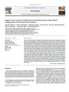
Figure 1: Total error rates (in %) obtained by the MCOS on the synthetic data represented in (a) for different number of clusters produced by the k-means clustering algorithm on a dataset of: (b) 100 samples, (c) 200 samples and (d) 400 samples.
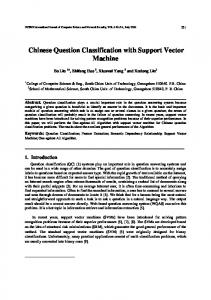
Figure 2: Example of clusters and decision boundaries obtained by the MCOS algorithm. Target samples are represented by ‘∗’ marks and outliers by ‘×’ marks. The samples and the contour of each training cluster are represented by the same color. Figure (a) represent the case with one cluster, (b) two clusters, (c) three clusters and (d) four clusters.
In the synthetic dataset, the target class is composed of two 2-D equiprobable Gaussians with different means and variances (PDF1 Ã N (µ = (1, 0), Σ = 0.25I), PDF2 Ã N (µ = (6, 0), Σ = I)), and the outlier class is composed of another Gaussian (N (µ = (3, 0), Σ = I)) between the two first ones, where I is the identity matrix. In order to simulate a realistic situation, the target samples represent 4/5 of the data and 1/5 of the data are outlier samples. Figure 1.a shows an example of this data with 200 samples. In addition to the clustering method and the number of clusters, the MCOS depends on the same parameters as the OCSVM: the kernel function K, the kernel parameter and only´the Gausthe regularization parameter ν . In this study, ³ kx−yk2 sian kernel of width σ , K(x, y) = exp − 2σ 2 , is considered as it has been widely reported in the literature to be the most suitable for one-class classification compared to other kernel functions such as Linear, Polynomial or Sigmoidal [20, 1, 16, 22]. Furthermore, because of the need for data separation from the origin, only Radial Basis Function (RBF) kernels such as the Gaussian Kernel can be used with the OCSVM algorithm [15]. For all the compared methods, a simple grid search with internal 3 fold cross-validation technique is used for the selection of the classifiers parameters by optimization of the validation TER. The values used for the width parameter σ and the regularization parameter ν are as follows: σ : {0.01, 0.1, 1, 3, 5, 8, 10, 12, 15, 17, 20}; ν : {0.01, 0.02, 0.05, 0.01, 0.2, 0.3, 0.5}. Integers from 1 to 10 are tested for the number of clusters. Averaged total error rates (TERs) estimated by using 5 runs of 5 fold cross-validation, are used to measure the performance of the MCOS algorithm. Figure 1 shows plots of Averaged TERs in function of the number of clusters for three data sets of 100, 200 and 400 samples respectively. For the number of clusters going from 1 to 10, plots of TERs are represented for the MCOS with the k-means algorithm. The single-cluster case corresponds to the standard OCSVM al-
gorithm. The theoretical Bayesian error probability is 7.22%. In the three cases of Figure 1, the OCSVM algorithm (MCOS algorithm with one training data cluster) always gives poor performance. This is expected, since the OCSVM algorithm using the same kernel on all training samples is not appropriate to represent this data which is composed of two clusters with different variances. Interestingly, however, the best performance for the three cases are obtained by the MCOS algorithm with 3,4 or 6 clusters, even though the target class was generated using two Gaussians. An explanation is that, because of the limitations of sampling, a finite dataset drawn from this distribution may have some irregularities, making it more appropriate to represent the target data with more than two clusters. For example, Figure 2 shows an example of clusters and decision boundaries obtained by the MCOS 1, 2, 3 and 4 training clusters are considered. In the case of 4 clusters (Figure 2.d), we can see that the three clusters, representing the right Gaussian of the target class, define three different subsets of the training samples that happen to have different densities. For each cluster, a different representation is optimized. Note from Figure 2(a), that the conventional OCSVM (equivalent to MCOS with one cluster) produces a poor representation of the data with a broad contour for the left cluster and an irregular contour for the right cluster. Here, the OCSVM uses the same kernel width σ = 0.5 on the two clusters of the training set which have different variances, 0.25 and 1 for left and right clusters respectively. In Figure 2(b), the representation by MCOS with two clusters is smoother and better fitted to the data structure with a small contour on the smaller cluster and a large contour on the larger cluster. In Figure 2(c), the larger cluster is represented by two contours and in Figure 2(d), it is represented by three contours. As the number of contours increases, we obtain a representation that is more closely tied to the training set as we can see on Figure 2(d) where the three right contours reproduce the shape of the largest cluster quite closely. By increasing the num-
1191
Total Error Rate (%)
36
Table 1: Averaged percentage TERs obtained on several real world datasets. For each dataset class, the best TER obtained by 5×5 fold cross-validation and the optimal number of clusters are displayed for: MCOSd and MCOSk with searched number of clusters k, and MCOSd and MCOSk with k being estimated by using the Gap Statistic algorithm. For each dataset class, the performances that are better than the OCSVM one are presented in bold.
32
28
24
20
2
4
6
8
10
Number of clusters
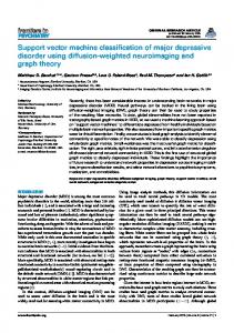
Figure 3: Performance of the MCOS with k-means clustering algorithm on the Glass database where class ‘2’ is considered as the outlier class and the other classes all together are considered as the target class.
ber of clusters, we will end up by having a contour on each training point and hence an extreme overfitting of the representation to the training set. Note that all the TER curves in Figure 1 have a generally convex shape. For small numbers of clusters, the model does not fit the data structure, and for large values, the model over-fits the training data which results in bad generalization performance in both cases. The graphs show that the number of clusters at which overfitting begins, grows with the size of the training set, which makes sense: because of the availability of more samples to build more local representations, bigger training sets can be represented with more clusters. In another example, we have considered the Glass database of the UCI Machine Learning Repository [3]. The Glass database is composed of six classes {1, 2, 3, 5, 6, 7} where in this example the class ‘2’ is considered as the outlier class and the other classes all together are considered as the target class. Figure 3 represents averaged values of TERs obtained by MCOS with k-means and shows a clear improvement of this algorithm over the performance of OCSVM. Note that the optimal number of clusters is different, though close, from the number of sub-classes (sub-distributions) of the target class which is 5. 6. EXPERIMENTS WITH REAL WORLD DATA This section presents classification results from experiments performed on nine databases from the UCI Machine Learning Repository [3]: Iris, Breast-Cancer, Glass, Haberman, Pima, Sonar,Balance, Wine and Spam. For each dataset, each of the classes is considered as the “Target”, at once, and all the other ones as “Outliers”. 5 runs of 5 fold crossvalidation are performed for total error rate estimation. As was done in the synthetic dataset experiments, a simple grid search with internal 3-fold cross-validation procedure is used for the selection of the classifiers’ parameters, and the Gaussian kernel function was used in all of the experiments. The following values where used for the kernel width σ : {0.01, 0.1, 1, 3, 5, 8, 10, 12, 15, 17, 20} for the Iris, Wine, Glass, Sonar and Haberman databases, and the following set of values {1, 3, 7, 10, 20, 30, 40, 50, 60, 80, 100} for the Pima and Haberman datasets which have a bigger range. The values {0.01, 0.02, 0.05, 0.2, 0.3, 0.5} were considered for the regularization parameter ν . Different values of the number of clusters are also tested ranging from 1 to to 25. In order to test the effect of using different clustering
OCSVM
Data(class) Iris(Setosa) Iris(Virgin.) Iris(Versico.) B.Cancer(B.) B.Cancer(M.) Glass(1) Glass(2) Glass(3) Glass(5) Glass(6) Glass(7) Haberman(1) Haberman(2) Pima(0) Pima(1) Sonar(M) Sonar(R) Balance(L) Balance(R) Wine(A) Wine(B) Wine(C) Spam(0) Spam(1)
Optimized k MCOSk
MCOSd
Pre-estimated k MCOSk
MCOSd
00.66 00.66(1) 00.66(1) 00.66(1) 00.66(1) 08.53 07.33(2) 07.79(3) 08.53(1) 08.53(1) 07.73 07.73(1) 06.53(2) 07.73(1) 07.73(1) 03.66 03.57(2) 03.13(3) 03.78(6) 03.94(6) 04.97 04.78(2) 04.97(1) 04.97(1) 04.97(1) 21.57 16.69(2) 16.62(2) 21.57(1) 21.57(1) 27.95 25.66(9) 26.13(4) 27.95(1) 27.95(1) 07.65 07.65(1) 07.65(1) 07.65(1) 07.65(1) 02.71 02.71(1) 02.71(1) 02.71(1) 02.71(1) 02.98 02.98(1) 02.98(1) 02.98(1) 02.98(1) 04.01 04.01(1) 03.82(2) 04.01(1) 04.01(1) 26.14 24.84(3) 25.69(2) 26.14(1) 26.14(1) 27.82 25.62(5) 26.34(7) 27.82(1) 27.82(1) 30.76 29.73(7) 27.47(11) 30.76(1) 30.76(1) 34.97 29.60(10)28.65(21) 34.97(1) 34.97(1) 38.36 24.80(16)25.43(12)30.18(5)32.24(5) 43.20 34.04(16)40.44(20)42.90(3)38.95(3) 09.69 09.69(1) 09.69(1) 15.26(4) 14.11(4) 09.43 09.43(1) 09.43(1) 13.76(4) 13.82(4) 12.37 11.70(2) 12.03(6) 12.37(1) 12.37(1) 23.56 20.54(5) 19.16(5) 23.56(1) 23.56(1) 11.35 09.52(2) 09.52(2) 11.35(1) 11.35(1) 30.30 26.06(7) 26.01(10) −− −− 29.80 25.19(7) 26.77(9) −− −−
methods, classification results are presented for the two cases where the k-means clustering algorithm and the Dendogarm based one, which is presented in Section 4.2, are used. We refer to the two cases by MCOSk and MCOSd respectively. For the target classes of each dataset, the average TERs which were obtained with OCSVM, MCOSk and MCOSd , are displayed in Table 1. The number of clusters that led to the best averaged error rate is also stated in parentheses for the two MCOS methods. In order to show the difficulty to estimate a priori the number of clusters for MCOS, the same information, except for the Spam database, are given for the case where the number of clusters k is estimated by using the Gap statistic algorithm [21] (referred to as ’Pre-estimated k’). The Gap statistic algorithm depends on the variance function given by Equation 3, and considers the gap between the observed value of this function and another value that is estimated over a number of datasets drawn from a reference distribution that could be uniform for example, see [21] for more details. In Table 1, for clarity, all the cases that improve upon the OCSVM performance are presented in bold. Table 1 shows in many cases that the MCOS is able to improve over the performance of OCSVM such as in the case of class ‘1’ of Glass (around 18% of error rate with MCOS compared to 24% with OCSVM), class ‘1’ of Pima (around 29% of error rate with MCOS compared to 35% with
1192
OCSVM), class ‘M’ of Sonar (around 25% of error rate with MCOS compared to 38% with OCSVM) and class ‘B’ of Wine database (around 19% of error rate with MCOS compared to 23% with OCSVM). Note that the performances of the two MCOS methods are very close for almost all the cases except for some cases such as the ‘R’ class of the Sonar database (34.04% of TER for MCOSk against 40.44% for MCOSd ) and class ‘0’ of Pima database (27.47% of TER for MCOSd against 29.73% for MCOSk ). However, the optimal numbers of clusters used by the k-means and the dendogram clustering methods are generally different, and the difference can be substantial, as in the case of class ‘2’ of Glass (the number of clusters k equals 9 for k-means against 4 for dendogram) and class ‘1’ of Pima database (k = 10 for k-means against k = 21 for dendogram). This indicates that it is difficult to predict a priori the optimal number of clusters as it depends on the used clustering method. This also means that the optimal number of clusters is different from the underlying number of subsets of the target class, as was shown on the two synthetic examples of Section 5, since it is not unique. 7. CONCLUSIONS In this paper, we have presented the Multi-Cluster One-Class Support Vector Machine (MCOS), which aims to overcome the poor performance of One Class Support Vector Algorithms when applied to multi-distributed data. Algorithms such as OCSVM and SVDD use the same kernel width on all support vectors, regardless if they are located in a dense region of the data distribution or in a sparse one. To overcome this weakness, the MCOS algorithm first uses a clustering algorithm to divide the training sets into coherent clusters, and then builds a OCSVM with a separate kernel on each cluster. The final representation of the data is then obtained by the combination of all the local representations. Our experiments on synthetic and real world data sets show that in many cases, by adapting the representation to the local characteristics of the data, the MCOS can offer clear improvement over the OCSVM performance. However, for some problems, MCOS cannot improve on OCSVM, but since it includes OCSVM as a special case, it is never worse than OCSVM. For future work, we will consider the problem of prior estimation of the optimum number of clusters for a given classification problem. In our experiments we have adopted a search method and show that in many cases this approach leads to considerable improvement compared to the the Gap Statistic approach, from data discovery domain, that consists of pre-estimating the number of clusters. Since the aim here is data classification, more adapted clustering methods, that take into account both the distributions of target and outlier classes, need to be searched. REFERENCES [1] H. Alashwal, S. Deris, and R. Othman. One-class support vector machines for protein-protein interactions prediction. International Journal of Biomedical Sciences, 1(2):120–127, 2006. [2] D. Arthur and S. Vassilvitskii. k-means++: the advantages of careful seeding. In SODA ’07: Proceedings of the 18th ACM-SIAM Symposium on Discrete Algorithms, pages 1027–1035, Philadelphia, USA, 2007.
[3] A. Asuncion and D. Newman. UCI machine learning repository. 2007. University of California, Irvine, School of Information and Computer Sciences. [4] L. Bottou and V. Vapnik. Local learning algorithms. Neural Computation, 4:888–900, 1992. [5] P. S. Bradley and U. M. Fayyad. Refining initial points for k-means clustering. In Proceedings of the Fifth International Conference on Machine Learning, pages 91–99. Morgan kaufmann, 1998. [6] T. Cover and P. Hart. Nearset neighbor pattern classification. IEEE Transactions in Information Theory, 13:21–27, 1967. [7] J. Hartigan and M. Wong. A K-means clustering algorithm. Applied Statistics, 28:100–108, 1979. [8] A. K. Jain and R. C. Dubes. Algorithms for clustering data. Prentice-Hall, Inc., U. S. R., NJ, USA, 1988. [9] L. Kaufman and P. J. Rousseeuw. Finding Groups in Data: an Introduction to Cluster Analysis. John Wiley & Sons Ltd, Chinchester, New York, 1990. [10] S. P. Lloyd. Least squares quantization in pcm. IEEE Trans. Information Theory, 28:129–137, 1982. [11] J. B. Macqueen. Some methods of classification and analysis of multivariate observations. In Proceedings of the Fifth Berkeley Symposium on Mathematical Statistics and Probability, pages 281–297, 1967. [12] J. Moody and C. J. Darken. Fast learning in networks of locally-tuned processing units. Neural Computation, 1(2), 1989. [13] R. A. Redner and H. F. Walker. Mixture densities, maximum likelihood and the em algorithm. SIAM Review, 26(2):195–239, 1984. [14] S. R. Sain. Adaptive Kernel Density Estimation. PhD thesis, Rice University, Texas, 1994. [15] B. Sch¨olkopf, J. Platt, J. Shawe-Taylor, A. J. Smola, and R. Williamson. Estimating the support of a high-dimentional distribution. Neural Computation, 13:1443–1471, 2001. [16] K.-K. Seo. An application of one-class support vector machines in content-based image retrieval. Expert Systems with Applications, 33(2):491–498, August 2007. [17] J. Shawe-Taylor and N. Cristianini. Support Vector Machines and other kernel-based learning methods. Cambridge University Press, 2000. [18] J. Shawe-Taylor and N. Cristianini. Kernel Methods for Pattern Analysis. Camb. Univ. Press, 2004. [19] D. Tax and R. Duin. Support vector domain description. Pattern Recognition Letters, 20:1191–1199, 1999. [20] D. Tax and R. Duin. Support vector data description. Machine Learning, 54:45–66, 2004. [21] R. Tibshirani, G. Walther, and T. Hastie. Estimating the number of clusters in a data set via the gap statistic. Journal of Royal Statistical Society B, 63(2):411–423, 2001. [22] H. Xu and D.-S. Huang. One class support vector machines for distinguishing photographs and graphics. In IEEE International Conference on Networking, Sensing and Control, 2008, pages 602–607, 2008.
1193