support vector regression with its application to short-term ... - CiteSeerX

Neural Networks 57 (2014) 1–11

Contents lists available at ScienceDirect

Neural Networks journal homepage: www.elsevier.com/locate/neunet

Noise model based ν -support vector regression with its application to short-term wind speed forecasting Qinghua Hu a,b,∗ , Shiguang Zhang a,c , Zongxia Xie d , Jusheng Mi a,e , Jie Wan f a

College of Mathematics and Information Science, Hebei Normal University, Shijiazhuang, Hebei, 050024, China

b

School of Computer Science and Technology, Tianjin University, Tianjin, 300072, China

c

College of Mathematics and Computer Science, Hengshui University, Hengshui, Hebei, 053000, China

d

School of Computer Software, Tianjin University, Tianjin, 300072, China

e

Hebei Key Laboratory of Computational Mathematics and Applications, Shijiazhuang, Hebei, 050024, China

f

School of Energy Science and Engineering, Harbin Institute of Technology, Harbin, 150001, China

article

info

Article history: Received 17 September 2013 Received in revised form 9 March 2014 Accepted 1 May 2014 Available online 13 May 2014 Keywords: Support vector regression Noise model Loss function Inequality constraints Wind speed forecasting

abstract Support vector regression (SVR) techniques are aimed at discovering a linear or nonlinear structure hidden in sample data. Most existing regression techniques take the assumption that the error distribution is Gaussian. However, it was observed that the noise in some real-world applications, such as wind power forecasting and direction of the arrival estimation problem, does not satisfy Gaussian distribution, but a beta distribution, Laplacian distribution, or other models. In these cases the current regression techniques are not optimal. According to the Bayesian approach, we derive a general loss function and develop a technique of the uniform model of ν -support vector regression for the general noise model (N-SVR). The Augmented Lagrange Multiplier method is introduced to solve N-SVR. Numerical experiments on artificial data sets, UCI data and short-term wind speed prediction are conducted. The results show the effectiveness of the proposed technique. © 2014 Elsevier Ltd. All rights reserved.

1. Introduction Regression is an old topic in the domain of learning functions from a set of samples (Hastie, Tibshirani, & Friedman, 2009). It provides researchers and engineers with a powerful tool to extract hidden rules of data. The trained model is used to predict future events with the information of past or present events. Regression analysis is now successfully applied in nearly all fields of science and technology, including the social sciences, economics, finance, wind power prediction for grid operation. However this domain is still attracting much attention from research and application domains. Generally speaking, there are three important issues in designing a regression algorithm: model structures, objective functions and optimization strategies. The model structures include linear or nonlinear functions (Park & Lee, 2005), neural networks (Spech,

1990), decision trees (Esposito, Malerba, & Semeraro, 1997), and so on; optimization objectives include ϵ -insensitive loss (Cortes & Vapnik, 1995; Vapnik, 1995; Vapnik, Golowich, & Smola, 1996), squared loss (Suykens, Lukas, & Vandewalle, 2000; Wu, 2010; Wu & Law, 2011), robust Huber loss (Olvi & David, 2000) etc. According to the formulation of optimization functions, a collection of optimization algorithms (Ma, 2010) have been developed. In this work, we focus on the problem which optimal formulation should be considered with respect to different error models. Suppose we are given a set of training data Dl = {(x1 , y1 ), (x2 , y2 ), . . . , (xl , yl )},

(1)

where xi ∈ R , yi ∈ R, i = 1, 2, . . . , l. Take a multivariate linear regression task f as an example. The form is L

f (x) = ωT · x + b,

(2)

where ω ∈ R , b ∈ R, i = 1, 2, . . . , l. The task is to learn the parameter vectors ω and parameter b, by minimizing the objective function L

∗ Corresponding author at: College of Mathematics and Information Science, Hebei Normal University, Shijiazhuang, Hebei, 050024, China. Tel.: +86 22 27401839. E-mail address: [email protected] (Q. Hu). http://dx.doi.org/10.1016/j.neunet.2014.05.003 0893-6080/© 2014 Elsevier Ltd. All rights reserved.

gLR =

l  (yi − ωT · xi − b)2 . i =1

(3)

2

Q. Hu et al. / Neural Networks 57 (2014) 1–11

where ξi , ξi∗ are two slack variables. The constant C > 0 determines the trade-off between the flatness of f and the amount up to which deviations larger than ϵ are tolerated. ν ∈ (0, 1] is a constant which controls the number of support vectors. In the ν -SVR the size of ϵ is not given a priori but a variable. Its value is traded off against the model complexity and slack variables via a constant ν (Chalimourda et al., 2004). This corresponds to dealing with a socalled ϵ -insensitive loss function (Cortes & Vapnik, 1995; Vapnik, 1995) described by cϵ (ξ ) = |ξ |ϵ =



0, |ξ | − ϵ,

if |ξ | ≤ ϵ, otherwise.

(5)

In 2002, ϵ -SVR for a general noise model was proposed in Schölkopf and Smola (2002):

 min gϵ -SVR =

1 2

 2

∥ω∥ + C ·

l 

Subject to :

ω T · xi + b − y i ≤ ϵ + ξ i

Fig. 1. Gaussian PDF and beta PDF of parameters.

The objective function of the sum-of-squares error is usually used in regression. The trained model is optimal, if the samples have been corrupted by independent and identical probability distributions (i.i.d.). Noise satisfying Gaussian distribution with zeros mean and variance σ 2 , i.e., yi = f (xi ) + ξi , i = 1, . . . , l, ξi ∼ N (0, σ 2 ). In the recent years, the support vector regressor (SVR) is growing up as a popular technique (Cortes & Vapnik, 1995; Cristianini & Shawe, 2000; Smola & Schölkopf, 2004; Vapnik, 1995, 1998, 1999; Vapnik et al., 1996; Wu, 2010; Wu & Law, 2011). It is a universal regression machine based on the V–C dimension theory. This technique is developed with the Structural Risk Minimization (SRM) principle, which has shown its effectiveness in applications. The classical SVR is optimized by minimizing Vapnik’s ϵ -insensitive loss function of residuals and has achieved good performance in a variety of practical applications (Bayro-Corrochano & Arana-Daniel, 2010; Duan, Xu, & Tsang, 2012; Huang, Song, Wu, & You, 2012; Kwok & Tsang, 2003; Lopez & Dorronsoro, 2012; Yang & Ong, 2011). In 1995, ϵ -SVR was proposed by Vapnik and his research team (Cortes & Vapnik, 1995; Vapnik, 1995; Vapnik et al., 1996). In 2000, ν -SVR was introduced by Schölkopf, Smola, Williamson, and Bartlett (2000), which automatically computes ϵ . Suykens et al. (2000) constructed least squares support vector regression with Gaussian noise (LS-SVR). Wu (Wu, 2010; Wu & Law, 2011) and Pontil, Mukherjee, and Girosi (1998) constructed ν -support vector regression with Gaussian noise (GN-SVR). If the noise obeys the Gaussian distribution, the outputs of the models are optimal. However, it was found that the noise in some real-world applications, just like wind power forecast and direction-of-arrival estimation problem, does not satisfy Gaussian distribution, but a beta distribution or Laplace distribution, respectively. In these cases these regression techniques are not optimal. The principle of ν -support vector regression (ν -SVR) can be written as (Chalimourda, Schölkopf, & Smola, 2004; Chih-Chung & Chih-Jen, 2002; Schölkopf et al., 2000):

 min gPν -SVR =

1 2

 ∥ω∥ + C · νϵ + 2

l 1

l i =1

Subject to :

ωT · xi + b − yi ≤ ϵ + ξi yi − ωT · xi − b ≤ ϵ + ξi∗

ξi , ξi∗ ≥ 0,

i = 1, 2, . . . , l, ϵ ≥ 0,



(ξi + ξi ) ∗

(4)

  c (ξi ) + c (ξi ) ∗

i=1

(6)

yi − ωT · xi − b ≤ ϵ + ξi∗

ξi , ξi∗ ≥ 0,

i = 1, 2, . . . , l,

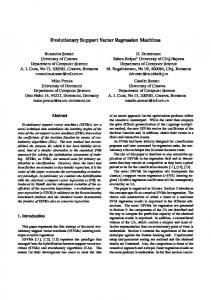
where c (x, y, f (x)) =  c (|y − f (x)|ϵ ) is a general convex loss function in the sample point (xi , yi ) of Dl . |y − f (x)|ϵ in (5) is Vapnik’s ϵ -insensitive loss function. Using Lagrange multiplier techniques (Cortes & Vapnik, 1995; Vapnik, 1995), Problem (4) can be transformed to a convex optimization problem with a global minimum. At the optimum, the l ∗ regression estimate takes the form f (x) = i=1 (αi −αi )(xi · x)+ b, where (xi · x) is the inner product. In 2002, Bofinger, Luig, and Beyer (2002) found that the output of wind turbine systems is limited between zero and the maximum power and the error statistics do not follow a normal distribution. In 2005, Fabbri, Román, Abbad, and Quezada (2005) believed that the normalized produced power p must be within the interval [0, 1] and the beta function is more appropriate to fit the error than the standard normal distribution function. Bludszuweit, Antonio, and Llombart (2008) showed the advantages of using the beta probability distribution function (PDF), instead of the Gaussian PDF, for approximating the forecast error distribution. The error ϵ between the predicted values xp and the measured values xm obeys the beta distribution in the forecast of wind power, and the PDF of ϵ is f (ϵ) = ϵ m−1 ·(1 −ϵ)n−1 · h, ϵ ∈ (0, 1), the parameters m and n are often called hyperparameters because they control the distribution of the variable ϵ (m > 1, n > 1), h is the normalization factor and parameters m and n are determined by the values of the mean (which is the predicted power) and the standard deviation (Bishop, 2006; Canavos, 1984). Fig. 1 shows plots of Gaussian distribution and the beta distribution for different values of hyperparameters. In 2007, Zhang, Wan, Zhao, and Yang (2007) and Randazzo, AbouKhousa, Pastorino, and Zoughi (2007) presented the estimation results under a Laplacian noise environment in the direction-ofarrival of coherent electromagnetic waves impinging estimation problem. Laplace distribution is frequently encountered in various machine learning areas, e.g., the over-complete wavelet transform coefficients of images, processing in Natural images, etc. (Eltoft, Kim, & Lee, 2006; Park & Lee, 2005). Based on the above analysis, we know that the error distributions do not satisfy Gaussian distribution in some real-world applications. We try to study the optimal loss functions for different error models. It is not suitable to apply the GN-SVR to fit functions from data with non-Gaussian noise. In order to solve the above problems,

Q. Hu et al. / Neural Networks 57 (2014) 1–11

we derive a general loss function and construct ν -support vector regression machines for a general noise model. Finally, we design a technique to find the optimal solution to the corresponding regression tasks. While there are a large number of implementations of SVR algorithms in the past years, we introduce the Augmented Lagrange Multiplier (ALM) method, presented in Section 4. If the task is non-differentiable or discontinuous, the sub-gradient descent method can be used (Ma, 2010), and if there are very large scale of samples, SMO can also be used (Shevade, Keerthi, Bhattacharyya, & Murthy, 2000). The main contributions of our work are listed as follows: (1) we derive the optimal loss functions for different error models by the use of Bayesian approach and optimization theory; (2) we develop the uniform ν -support vector regression model for the general noise with inequality constraints (N-SVR); (3) the Augmented Lagrange Multiplier method is applied to solve N-SVR, which guarantees the stability and validity of the solution in N-SVR; (4) we utilize N-SVR to short-term wind speed prediction and show the effectiveness of the proposed model in practical applications. This paper is organized as follows: in Section 2 we derive the optimal loss function corresponding to a noise model by using the Bayesian approach; in Section 3 we describe the proposed ν -support vector regression technique for general noise model (N-SVR); in Section 4 we give the solution and algorithm design of N-SVR; numerical experiments are conducted on artificial data sets, UCI data and short-term wind speed prediction in Sections 5 and 6; finally, we conclude the work in Section 7.

Given a set of noisy training samples Dl , we require to estimate an unknown function f (x). Following Chu, Keerthi, and Ong (2004); Girosi (1991); Klaus-Robert and Sebastian (2001); Pontil et al. (1998), the general approach is to minimize H [f ] =

c (ξi ) + λ · Φ [f ],

(7)

i =1

where c (ξi ) = c (yi − f (xi )) is a loss function, λ is a positive number and Φ [f ] is a smoothness functional. We assume the noise is additive yi = f (xi ) + ξi ,

i = 1, 2, . . . , l,

(8)

where ξi is random, independent, identical probability distributions (i.i.d.) with P (ξi ) of variance σ and mean µ. We want to estimate the function f (x) with the set of data Df ⊆ Dl . We take a probabilistic approach, and regard the function f as the realization of a random field with a known prior probability distribution. We are interested in maximizing the posteriori probability of f given the data Df , namely P [f |Df ], which can be written as P [f |Df ] ∝ P [Df |f ] · P [f ],

(9)

where P [Df |f ] is the conditional probability of the data Df given the function f and P [f ] is a priori probability of the random field f , which is often written as P [f ] ∝ exp(−λ · Φ [f ]), where Φ [f ] is a smoothness functional. The probability P [Df |f ] is essentially a model of the noise, and if the noise is additive, as in Eq. (8) and i.i.d. with probability distribution P (ξi ), it can be written as P [Df |f ] =

l 

P (ξi ).

Fig. 2. Loss function of the corresponding noise model.

minimizes the following functional H [f ] = −

l 

log[P (yi − f (xi )) · e−λ·Φ [f ] ]

i=1

=−

l 

log P (yi − f (xi )) + λ · Φ [f ].

(11)

i=1

2. Bayesian approach to the general loss function

l 

3

(10)

i =1

Substituting P [f ] and Eq. (10) in (9), we see that the function that maximizes the posterior probability of f is the one which

This functional is of the same form as Eq. (7) (Girosi, 1991; Pontil et al., 1998). By Eqs. (7) and (11), the optimal loss function in a maximum likelihood sense is c (x, y, f (x)) = − log p(y − f (x)),

(12)

i.e. the loss function c (ξ ) is the log-likelihood of the noise. We assume that the noise in Eq. (8) is Gaussian, with zero mean and variance σ . By Eq. (12), the loss function corresponding to Gaussian-noise is c (ξi ) =

1 2σ 2

(yi − f (xi ))2 .

(13)

If the noise in Eq. (8) is beta, with mean µ ∈ (0, 1) and variance σ , get m = (1−µ)·µ2 /σ 2 −µ, n = ((1−µ)/µ)·m (m > 1, n > 1), and h = Γ (m + n)/(Γ (m) · Γ (n)) is the normalization factor (Bofinger et al., 2002). By Eq. (12), the loss function corresponding to beta-noise is c (ξi ) = (1 − m) log(ξi ) + (1 − n) log(1 − ξi ),

(14)

where parameters m > 1, n > 1. And if the noise in Eq. (8) is Weibull, with parameters θ and k. By Eq. (12), the loss function should be

  

ξi (1 − k) log + c (ξi ) = θ  0,

 k ξi , θ

if ξi ≥ 0,

(15)

otherwise.

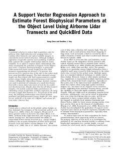
The loss functions and their corresponding probability density functions (PDF) of the noise models used in regression problems are listed in Table 1 and shown in Fig. 2. 3. Noise model based ν-support vector regression Given samples Dl , we construct a linear regression function f (x) = ωT · x + b. In order to deal with nonlinear functions the

4

Q. Hu et al. / Neural Networks 57 (2014) 1–11 Table 1 Loss function and PDF of the corresponding noise model. Function case

PDF of the noise model

Loss function

Laplace

P (ξi ) =

c (ξi ) = |ξi |

ϵ -insensitive

P (ξi ) =

P (ξi ) =

Exponent

1 −|ξi | e 2

   

1

, if |ξ | ≤ ϵ, 2(1 + ϵ) 1    eϵ−|ξi | , otherwise.  2(1 + ϵ) ξi 1  e− θ , if ξi ≥ 0, θ

0,

P (ξi ) =

Gauss

c (ξi ) = P (ξi ) =

Huber

−

p 2·Γ ( 1p )

e

|ξi |p

c (ξi ) =

p

ξ  ξ2 e− 2i , e

ϵ 2 −ϵ|ξ | i 2

ifξi ≤ ϵ,

,

c (ξi ) =

otherwise.

beta

P (ξi ) = ξim−1 · (1 − ξi )n−1 · h, h =

Weibull

  k−1 ξi k k x e−( θ ) , P (ξi ) = θ θ  0,

K (xi , xj ) = (Φ (xi ) · Φ (xj )).

otherwise.



 l 1 1 T ∗ (c (ξi ) + c (ξi )) = ω · ω + C · νϵ + l i =1

Subject to :

(17)

ω · Φ (xi ) + b − yi ≤ ϵ + ξi T

yi − ωT · Φ (xi ) − b ≤ ϵ + ξi∗

Theorem 1. The solution of the primal problem (17) of N-SVR about ω exists and is unique. Proof. It is trivial to prove the existence of the solution. The uniqueness of the solution certificate as follows. There are two ω,  b,  ξ ) in the primal problem (17). Define solutions (ω, b, ξ ) and ( (ω, b, ξ ) as 1 2

(ω +  ω),

b=

1 2

(b +  b),

ξ=

1 2

(ξ +  ξ ).

We have yi − ωT · Φ (xi ) − b − ξi = yi −

1 2

2

 ξ    ,

if ξi ≤ ϵ,

2

2   ϵ|ξi | − ϵ ,

=

1 2

if ξi ≥ 0, otherwise.

(yi − ωT · Φ (xi ) − b − ξ i ) 1

+ (yi −  ωT · Φ (xi ) −  b − ξi ) 2

= 0,

(19)

where ξi = 12 (ξi +  ξi ) ≥ 0, i = 1, . . . , l. Suppose (ω, b, ξ ) is a feasible solution of the primal problem (17). Then we have 1 2 1 2

∥ω∥2 +

∥ω∥2 +

l C 

l i=1 l C 

l i=1

c (ξi ) ≥

c (ξi ) ≥

1 2 1 2

∥ω∥2 +

∥ ω ∥2 +

l C 

l i =1 l C 

l i =1

c (ξ i ),

(20)

c ( ξi ).

(21)

By (20) and (21), we have 2∥ω∥2 ≥ ∥ω∥2 + ∥ ω∥2 . Substitute ω into the above inequalities 2ω = ω + 

∥ω +  ω∥2 ≥ 2(∥ω∥2 + ∥ ω∥2 ).

i = 1, 2, . . . , l, ϵ ≥ 0,

c (ξi ), c (ξi )∗ ≥ 0 (i = 1, 2, . . . , l) are general convex loss functions in the sample point (xi , yi ) ∈ Dl . C > 0 is a penalty parameter.

ω=

ξi2

  k  (1 − k) log ξi + ξi , c (ξi ) = θ θ   0,

if ξi ≥ 0,

We develop a technique of the uniform model of ν -support vector regression for the general noise model. The primal problem of N-SVR is described as

ξi , ξi∗ ≥ 0,

|ξi |p

otherwise. 2 c (ξi ) = (1 − m) log(ξi ) + (1 − n) log(1 − ξi )

Γ (m+n) Γ (m)·Γ (n)

(16)

2

if ξi ≥ 0, otherwise.

2·π 2 i

following generalization can be done (Schölkopf & Smola, 2002; Vapnik, 1995, 1998): we map the input vectors xi ∈ RL into a highdimensional feature space H through some nonlinear mapping, Φ : RL → H (H is Hilbert space), chosen a priori. We then solve the optimization problem (4) in the feature space H. In this case, the inner product of the input vectors (xi · x) is replaced by the inner product of their icons in feature space H (Φ (xi ) · Φ (xj )). By using a function K (•, •), the linear model is extended to a nonlinear support vector regression machine

min gPN-SVR

1 p

P (ξi ) = √ 1 e−

1 2 2 i





  ξi , c (ξi ) = θ  0,

otherwise.

 Polynomial

cϵ (ξi ) = |ξi |ϵ

(ω +  ω)T · Φ (xi )

1

1

2

2

− (b +  b) − (ξi +  ξi )

(22)

As ∥ω +  ω∥ ≤ ∥ω∥ + ∥ ω∥, by (22) we have

(∥ω∥ + ∥ ω∥)2 ≥ ∥ω +  ω∥2 ≥ 2(∥ω∥2 + ∥ ω∥2 ).

(23)

As 2∥ω∥ · ∥ ω∥ ≤ ∥ω∥2 + ∥ ω∥2 , by (23) we derive

ω∥ = ∥ω∥2 + ∥ ω ∥2 , 2∥ω∥ · ∥ = ∥ω∥ + ∥ ω∥.

∥ω∥ = ∥ ω∥,

∥ω +  ω∥

(18) Thus  ω = λ · ω. Therefore λ = 1 or λ = −1. If λ = −1, ω + ω = 0. Thus ∥ω +  ω∥ = ∥ω∥ + ∥ ω∥ = 0. So ∥ω∥ = ∥ ω∥ = 0, namely, ω =  ω = 0. If λ = 1, ω =  ω. To sum up, the solution of the primal problem (17) about ω exists and is unique.

Q. Hu et al. / Neural Networks 57 (2014) 1–11

To estimate ϵ for

Theorem 2. The dual problem of the primal problem (17) of N-SVR is

 max gDN-SVR = −

ϵ=

l l 1 

2 i=1 j=1

(αi − αi ) · (αj − αj ) · K (xi , xj )

l

∗

∗

 C  + (αi∗ − αi ) · yi + (T (ξi (αi )) + T (ξi∗ (αi∗ )))

ϵ=

l i=1

i =1

Subjected to (24)

l  (αi∗ − αi ) = 0

(∗)

≤

C l

,

 (αi∗ + αi ) ≤ C · ν,

i = 1, 2, . . . , l

i=1

(∗)

(αi(∗) )) = c (ξi(∗) (αi(∗) ))−ξi(∗) (αi(∗) )·

(∗)

∂(c (ξi

(∗)

∂(ξi

0, 0 < ν ≤ 1 is constant.

(∗)

(αi ))) (∗)

(αi ))

,C>

Proof. We introduce the Lagrange functional L(ω, b, α, α ∗ , ξ , ξ ∗ , η, η∗ , ϵ) as 1

L =

2



l 

l i =1

(ηi ξi + ηi∗ ξi∗ ) −

l 

i=1

−

l 

(c (ξi ) + c (ξi∗ )) − γ ϵ

l 1

l k =1

∇b (L) = 0,

∇ϵ (L) = 0,

∇ξ (∗) (L) = 0.

l  (αi∗ − αi ) = 0,

i =1

i=1

 max gDν -SVR = −

∂(ξi )

+

ωi =

(αi∗ − αi ) · Φ (xi ),

+

 k=1

(αi∗ − αi )(αj∗ − αj )K (xi , xj )

(αi − αi ) · yi ∗

(25)

≤

C l

,

i = 1, . . . , l

l  (αi + αi∗ ) ≤ C · ν,

i = 1, . . . , l.

i=1

(2) Gaussian noise model GN-SVR: Suykens et al. (2000); Wu (2010); Wu and Law (2011) studied the support vector regression machine with equality constraints, inequality constraints, respectively. The function corresponding to Gaussian noise is c (ξi ) = ξi2 /2. Thus the dual problem for the Gaussian noise model is





1  

(αi∗ − αi )(αj∗ − αj )K (xi , xj )

2 i∈RSV j∈RSV

(αi − αi )yi −

l l 

∗

2C i=1



(α + (αi ) ) ∗ 2

2 i

yj −

 i∈RSV

 yk −



(αi − αi ) · K (xi , xj ) 

(αi − αi ) · K (xi , xk )

i∈RSV

i=1

(∗)

0 ≤ αi

≤

C l

,

i = 1, . . . , l i = 1, . . . , l.

i=1

∗

∗

(26)

l  (αi∗ − αi ) = 0

l  (αi + αi∗ ) ≤ C · ν,



j =1 l

2 i∈RSV j∈RSV

Subject to

  l 1  2l

1  

i∈RSV

i∈RSV

b =

(αi∗ − αi )K (xi , x) + b,

l  (αi∗ − αi ) = 0

+

− ηi(∗) − αi(∗) = 0.

Substituting the extreme conditions into L and seeking maximum of α, α ∗ , we obtain the dual problem (24) of the primal problem (17). We have





 

i =1

l

(αi − αi ) · K (xi , xk ) − b .

i∈RSV

max gDGN-SVR = −

l  C ·ν−γ − (αi∗ + αi ) = 0,

(∗)

yk −

∗

where RSVs are the samples corresponding to αi∗ − αi ̸= 0 (called support vectors). The dual problem (24) of ν -SVR, GN-SVR, HN-SVR and BN-SVR is described as follows. (1) ν -SVR: In Chalimourda et al. (2004), Chih-Chung and ChihJen (2002) and Spech (1990), the loss function for sample point (xi , yi ) ∈ Dl is c (ξi ) = ξi , the dual problem of ν -SVR is

(∗)

l  (αi∗ − αi ) · Φ (xi ),

∂(c (ξi(∗) ))

 

Then the decision-making function of ν -support vector regression with inequality constraints (N-SVR) can be written as

0 ≤ αi

And we get

·



i=1

αi∗ (ξi∗ − yi + ωT · Φ (xi ) + b + ϵ).

To minimize L, we derive partial derivatives ω, b, ξ , ξ ∗ , ϵ , respectively. According to the KKT (Karush–Kuhn–Tucker) conditions, we have

C

i∈RSV

Subject to

αi (ξi + yi − ωT · Φ (xi ) − b + ϵ)

i=1

ωi =

(αi − αi ) · K (xi , xj ) + b − yj , ∗

i∈RSV

i=1

∇ω (L) = 0,

l j=1



l 1

ωT · ω + C · νϵ +

−

 

i∈RSV

i = 1, 2, . . . , l

l

where T (ξi



f (x) = ωT · Φ (x) + b =

i=1

0 ≤ αi

l 1

or



l

5

(3) HN-SVR for  the Robust model: The robust Huber loss func-

 ξi

2

.

tion is c (ξi ) =

2



,

ϵ|ξi | −

if ξi ≤ ϵ,

ϵ

2

2

,

otherwise.

(Huber, 1964, 1981; Olvi &

6

Q. Hu et al. / Neural Networks 57 (2014) 1–11

4. Solution based on the Augmented Lagrange Multiplier method

David, 2000; Vapnik, 1995). The dual problem of HN-SVR is

 max gDHN-SVR = −



+

1  

(αi∗ − αi ) · (αj∗ − αj ) · K (xi , xj )

2 i∈RSV j∈RSV

(αi − αi ) · yi −

i∈RSV



l l 

∗

2C i=1

(α + (αi ) ) ∗ 2

2 i

Subject to (27)

l  (αi∗ − αi ) = 0 i =1

(∗)

0 ≤ αi

≤

Cϵ l

,

Theorems 1 and 2 supply an algorithm to effectively recognize the model of N-SVR. We obtain the solution based on the Augmented Lagrange Multiplier (ALM) method and the algorithm design of ν -support vector regression machine with the noise model (N-SVR) in this section. (1) Let data set Dl = {(x1 , y1 ), (x2 , y2 ), . . . , (xl , yl )}, where xi ∈ RL , yi ∈ R, i = 1, . . . , l. (2) Use a 10-fold cross validation strategy to search the optimal parameters C , ν, m, n, and select a kernel function K (•, •). (3) Construct and solve the optimization problem

i = 1, . . . , l

 max gDN-SVR = −

l

 (αi + αi∗ ) ≤ C · ν,

i = 1, . . . , l.

i =1



+ (4) SVR for beta noise (BN-SVR): The loss function for beta noise is c (ξi ) = (1 − m) log(ξi ) + (1 − n) log(1 − ξi ), 0 < ξi < 1, m > ∂(c (ξ )) ∂(c (ξ )) −β − 11−ξ , by Cl ∂(ξ i) − αi = 0, 1, n > 1. On account of ∂(ξ i) = 1−α ξ i

i

i

i

we have (αi l/C )·ξ −(2 +αi l/C − m − n)·ξi + 1 − m = 0. We derive 2 i

1 2

2αi l/C 2αi l/C

i∈RSV

2 + αi l/C − m − n + ∆ ∗

,

2αi∗ l/C

1 2

1   2 i∈RSV i∈RSV

(αi∗ − αi )yi −

(∗)

where T (ξi

(αi∗ − αi )(αj∗ − αj )K (xi , xj )

i=1

i=1

i=1

 l  ∗ ∗ ∗ ∗ +C ((1 − m) log(ξi (αi )) + (1 − n) log(ξi (1 − αi ))) (28) i=1

Subjected to l  (αi∗ − αi ) = 0 i=1

(∗)

≤

C l

,

i = 1, . . . , l

l  (αi + αi∗ ) ≤ C · ν, i =1

C l

,

i = 1, . . . , l i = 1, . . . , l

(αi(∗) )) = c (ξi(∗) (αi(∗) ))−ξi(∗) (αi(∗) )·

ν ≤ 1, C > 0 is constant.

i = 1, . . . , l.

(∗)

∂(c (ξi

(∗)

∂(ξi

(∗)

(αi ))) (∗)

(αi ))

,0
1, n > 1.

+

l i =1

 ∗

l  (αi∗ − αi ) = 0

Analogically, let

max gDBN-SVR = −

l C 

l  (αi + αi∗ ) ≤ C · ν,

where ∆ = (αi l/C + m − n) + 4(1 + mn − m − n), m > 1, n > 1. As 0 < ξi (αi ) < 1, we reject ξi2 (αi ) and adopt ξi1 (αi ), let ξi (αi ) = ξi1 (αi ).



(αi∗ − αi )(αj∗ − αj )K (xi , xj )

Subject to

(∗)

2

ξi∗ (αi∗ ) =

(αi − αi )yi + ∗

0 ≤ αi

,

1

2 + αi l/C − m − n − ∆ 2

ξi2 (αi ) =

2 i∈RSV j∈RSV

i =1

2 + αi l/C − m − n + ∆

ξi1 (αi ) =

1  



1 2l

l

The ALM method is a class of algorithms for solving equality or inequality constrained optimization problems. For nonlinear programming problems with equality constraints, Powell and Hestenes (Rockafellar, 1973) designed a dual method of solution, where squares of the constraint functions are added as penalties to the Lagrangian, and a certain simple rule is used for updating the Lagrange multipliers after each cycle (called the PH algorithm). Rockafellar (1973, 1974) extended it for solving inequality constrained tasks (called the PHR algorithm). The algorithm starts from the Lagrange function of the original problem, coupled with an appropriate penalty function. The original problem is transformed into solving a series of unconstrained optimization sub-problems. The ALM method was employed to solve Problem (29) by applying Newton’s method to a sequence of equality and inequality constrained problems. Any equality and inequality constrained minimization problem can be reduced to an equivalent unconstrained problem by eliminating the equality and inequality constrains. The Gradient descent method or Newton’s method can be used to solve the problem (Boyd & Vandenberghe, 2004; Chen & Jian, 1994; Fiacco & McCormick, 1990; Ma, 2010). If there are large-scale training samples, some fast optimization techniques can also be combined with the proposed objective functions, such as stochastic gradient decent (SDG) (Bottou, 2010).

Q. Hu et al. / Neural Networks 57 (2014) 1–11

In this work, we solve the ν -support vector regression machine with the ALM algorithm. ALM is used to solve Problem (29) by applying Newton’s method to a sequence of equality and inequality constrained problems. Problem (29) is equivalent to min f (x) hi (x) = 0,

i = 1, . . . , L1

gi (x) ≥ 0,

i = 1, . . . , L2

(30)

Table 2 Error statistic of three models on artificial data with Gaussian noise. Model

MAE

RMSE

MAPE (%)

ν -SVR

1.1647 0.9860 1.0036

1.4670 1.2517 1.2651

36.59 27.88 28.54

GN-SVR BN-SVR

function are used in ν -SVR, GN-SVR and BN-SVR (Schölkopf & Smola, 2002). K (xi , xj ) = ((xi , xj ) + 1)d ,

with f (x) =

7

l l 1 

2 i=1 j=1

K ( xi , xj ) = e

(αi∗ − αi )(αj∗ − αj )K (xi , xj )

∥xi −xj ∥2 σ2

,

where d is a positive integer, and σ is positive.

l l  C  − (αi∗ − αi )yi − (T (ξi (αi )) + T (ξi∗ (αi∗ ))),

l i =1

i =1

(31)

where x = (α1 , α2 , . . . , αl , α1∗ , α2∗ , . . . , αl∗ ), and l is the number of training samples. Construct the augmented Lagrange function of Problem (30)

Ψ (x, µ, λ, σ ) = f (x) −

L1  i=1

+

µi hi (x) +

L1 σ  (hi (x))2

2 i=1

L2 1 

2σ i=1

([min{0, σ gi (x) − λi }]2 − λ2i ).

(32)

(µk+1 )i = (µk )i − σ hi (xk ), i = 1, . . . , L1 (λk+1 )i = max{0, (λk )i − σ gi (xk )}, i = 1, . . . , L2 .

(33)

Let

 L L2 1   [min{gi (xk ), (λk )i /σ }]2 βk =  (hi (xk ))2 +

5. Experimental analysis In this section, we present some experiments to test the proposed model on several regression tasks with artificial data and UCI data. The following criteria, including mean absolute error (MAE), mean absolute percentage error (MAPE), the root mean square error (RMSE), and the standard error of prediction (SEP), are introduced to evaluate the performance of the ν -SVR, GN-SVR and BN-SVR models: MAE =

Formulation iteration of the multiplier method is

i =1

−

(34)

MAPE =

Step 1 Selection starting value. Take x0 ∈ Rn , µ1 ∈ RL1 , λ1 ∈ RL2 , σ1 > 0, 0 ≤ ϵ ≪ 1, δ ∈ (0, 1), η > 1, k := 1. Step 2 Solve the Augment Lagrange function. Take starting point xk−1 , solve the minimum point xk of unrestrained subproblem Ψ (x, µk , λk , σk ) in (32). Step 3 Examine termination conditions. If βk ≤ ϵ in (34), end iteration (32), and get the approximate minimum point xk of optimization problem (29); otherwise, turn Step 4. Step 4 Update penalty parameter. If βk ≥ δβk−1 , take σk+1 = ησk ; otherwise, σk+1 = σk . Step 5 Update the multiplier vector. Calculation (µk+1 )i , (λk+1 )i in (33). Step 6 Take k := k + 1, turn Step 1. In the ALM algorithm, parameters µ1 = (0.1, 0.1, . . . , 0.1)T , λ1 = (0.1, 0.1, . . . , 0.1)T , σ1 = 0.4, ϵ = 10−5 , η = 2, δ = 0.8. N-SVR has been implemented in Matlab 7.1 programming language. The initial parameters of the proposed ALM method are C ∈ [1, 201], ν ∈ (0, 1], m, n ∈ (1, 21). We use the 10-fold cross validation strategy to search the optimal positive parameters C , ν, m, n, the selection technique of parameters C , ν, m, n was studied in detail in Chalimourda et al. (2004) and Cherkassky and Ma (2004). Many actual applications suggest that polynomial and Gaussian kernel function tend to perform well under general smoothness assumptions, so that it should be considered especially if no additional information is used as the kernel function of N-SVR. In this work, the polynomial function and the Gaussian kernel

l i=1

|yi − xi |,

l 1  |yi − xi |

l i=1

xi

(35)

,

  l 1  (yi − xi )2 , RMSE =  l i =1

i=1

the stopping rule is βk ≤ ϵ , where ϵ ≥ 0 is a given threshold. Finally, the algorithm of ALM is described as follows.

l 1

SEP =

RMSE x

,

(36)

(37)

(38)

where l is the size of the samples, xi is the ith sample and yi is the forecasting result of the ith data, x is the average of all the samples (Bludszuweit et al., 2008; Fan et al., 2009; Guo, Zhao, Zhang, & Wang, 2011). 5.1. Artificial data sets To illustrate N-SVR, artificial data sets with Gauss-noise and beta-noise are studied. (1) Artificial data with Gauss-noise: as a training set, we use 300 examples (xi , yi ), the relationships between inputs xi and targets yi are as follows: yi = 2 sin(3xi + 2) + 6 cos(2xi + 1) + norm(0, 1, 1000, 1), here the xi is drawn uniformly from the interval [0.01 × π , 10 × π ]. Let the number of training samples be 150 (from 1 to 150), and the number of tested samples be 150 (from 151 to 300). Fig. 3 gives the forecasting results of artificial data with Gaussian noise given by ν -SVR, GN-SVR and BN-SVR, respectively. The criteria of MAE, MAPE and RMSE are used to evaluate the forecasting performance of three models, shown in Table 2. It is easy to see that GN-SVR is better than ν -SVR and BN-SVR on the artificial data with Gaussian noise. (2) Artificial data with beta-noise: as a training set, we use 300 examples (xi , yi ), the relationships between inputs xi and targets yi are yi = 2 sin(3xi +2)+6 cos(2xi +1)+6 beta(1.41, 1.71, 1000, 1), where xi is drawn uniformly from the interval [0.01 × π , 10 × π ]. Let the number of training samples be 150 (from 1 to 150), and the number of tested samples be 150 (from 151 to 300). Fig. 4

8

Q. Hu et al. / Neural Networks 57 (2014) 1–11

Fig. 3. The forecast result of three models on artificial data with Gaussian noise. Fig. 5. The forecast result of three models on abalone data set.

Fig. 4. The forecast result of three models on artificial data with beta noise. Table 3 Error statistic of three models on artificial data with beta noise.

Fig. 6. The forecast result of three models on stock data set.

Model

MAE

RMSE

MAPE (%)

ν -SVR

1.5857 1.5580 1.1467

1.9154 1.8909 1.3965

17.857 18.378 11.325

GN-SVR BN-SVR

illuminates the forecast results of artificial data with beta noise given by ν -SVR, GN-SVR and BN-SVR. The criteria of MAE, MAPE and RMSE are used to evaluate the forecast results of three models shown in Table 3. Experimental results on artificial data with beta noise demonstrate that BN-SVR is better than the classical models. 5.2. UCI data sets UCI data include abalone and stock, etc. We first add beta-noise to two data sets above, let the number of training samples be 240 (from 1 to 240), and the number of tested samples be 480 (from 241 to 720). Figs. 5 and 6 illuminate the forecast results of abalone and stock data sets with beta noise given by ν -SVR, GN-SVR and BN-SVR, respectively. The criteria of MAE, MAPE and RMSE are used to evaluate the forecast results of three models shown in Tables 4 and 5. The experiment results on UCI data with beta noise show that BN-SVR is better than ν -SVR and GN-SVR.

Table 4 Error statistic of three models on abalone data set. Model

MAE

RMSE

MAPE (%)

ν -SVR

0.0932 0.0932 0.0892

0.1158 0.1164 0.1128

21.92 21.82 18.94

GN-SVR BN-SVR

Table 5 Error statistic of three models on stock data set. Model

MAE

RMSE

MAPE (%)

ν -SVR

0.0943 0.0938 0.0801

0.1142 0.1135 0.1002

14.27 14.39 11.34

GN-SVR BN-SVR

6. Short-term wind speed prediction with the proposed algorithm The forecasting model of N-SVR is applied in a real-world sample set of wind speed in Heilongjiang Province. The data record more than a year wind speeds. The average wind speeds in 10 min are stored. As a whole, 62 466 samples with 4 attributes, mean, variance, minimum, maximum, are given.

Q. Hu et al. / Neural Networks 57 (2014) 1–11

9

Fig. 9. The boxplot of three models on wind speed prediction after 10 min.

Fig. 7. The beta distribution of the wind speed forecasting error with the persistence method.

Fig. 10. The forecasting result of three models on wind speed after 60 min.

Fig. 8. The forecasting result of three models on wind speed after 10 min.

We analyze one-month time series of wind speeds. Let us investigate the error distribution by using the persistence method (Bludszuweit et al., 2008). The result shows that the error ϵ of wind speed with the persistence forecast does not obey the Gaussian distribution, while obeys the beta distribution, and the PDF of ϵ is f (ϵ) = ϵ 7.22 · (1 − ϵ)27.32 , ϵ ∈ (0, 1), as shown in Fig. 7. Now, we use 288 samples (from 1 to 288, the time length is 48 h) as a training set, and 576 samples as a test set (from 289 − → to 864, the time length is 96 h). The input vector is xi = (xi−11 , xi−10 , . . . , xi−1 , xi ), the output value is xi+step , where step = 1, 6. Namely we use the above model to predict the wind speed after 10 and 60 min of each point xi , respectively. Figs. 8–11 give the forecasting results given by ν -SVR, GN-SVR and BN-SVR. Figs. 8 and 9 illuminate the forecasting results after 10 min of every point xi given by ν -SVR, GN-SVR and BN-SVR. The indicators of MAE, MAPE, RMSE and SEP are shown in Table 6. Figs. 10 and 11 present the forecasting results after 60 min of every point xi given by ν -SVR, GN-SVR and BN-SVR. The indicators of MAE, MAPE, RMSE and SEP are shown in Table 7.

Fig. 11. The boxplot of three models on wind speed prediction after 60 min. Table 6 Error statistic of three models on wind speed prediction after 10 min. Model

MAE (m/s)

RMSE (m/s)

MAPE (%)

SEP (%)

ν -SVR

0.4485 0.4465 0.4391

0.5848 0.5823 0.5692

3.86 3.84 3.79

4.96 4.94 4.83

GN-SVR BN-SVR

From Box–whisker Plots 9 and 11, Figs. 8 and 10, Tables 6 and 7, it is to derive that the errors computed with BN-SVR are a little

10

Q. Hu et al. / Neural Networks 57 (2014) 1–11

Table 7 Error statistic of three models on wind speed prediction after 60 min. Model

MAE (m/s)

RMSE (m/s)

MAPE (%)

SEP (%)

ν -SVR

1.3388 1.3304 1.3206

1.5988 1.5912 1.5811

12.53 12.50 12.40

13.59 13.52 13.44

GN-SVR BN-SVR

smaller than those with ν -SVR and GN-SVR in the most cases. As the prediction horizon increases to 60 min, both the errors derived with different models rise, the relative difference decreases. So it is not so significant in these cases. However, we can know Beta model is still better than the classical models in terms of all the criteria of MAE, MAPE, RMSE and SEP, seen from Tables 6 and 7. 7. Conclusions and future work Most existing regression techniques take the assumption that the error model is Gaussian. However, it was found that the noise in some real-world applications, just like wind speed forecast, does not satisfy Gaussian distribution, but a beta distribution. In this case, these regression techniques are not optimal. In this work, we describe the main results of our work: (1) we derive the optimal loss functions for different error models; (2) we develop the uniform ν -support vector regression for the general noise model (N-SVR); (3) the solution of the primal problem of N-SVR about ω exists and is unique; (4) introducing the Lagrange functional and according to KKT conditions, we obtain the dual problem of N-SVR; (5) the Augmented Lagrange Multiplier method is applied to solve N-SVR, which guarantees the stability and validity; (6) experimental results on artificial data sets, UCI data and the real-world data of wind speed confirm the performance of the proposed technique. Similarly, we can derive the model of ν -support vector classification for the general noise model, which will be successfully used to solve the classification problem for the noise model. In practical regression problems, data uncertainty is inevitable. The observed data are usually described in linguistic levels or ambiguous metrics. Like the weather forecast, the forecast results of dry and wet, or sunny and cloudy, and so on. We should consider developing fuzzy ν -support vector regression algorithms with different noise models. Acknowledgments This work was supported by National Program on Key Basic Research Project (973 Program) under Grant 2012CB215201, and National Natural Science Foundation of China (NSFC) under Grants 61222210, 61170107, 61105054, and 61300121. References Bayro-Corrochano, E. J., & Arana-Daniel, N. (2010). Clifford support vector machines for classification, regression, and recurrence. IEEE Transactions on Neural Networks, 21(11), 1731–1746. Bishop, C. M. (2006). Pattern recognition and machine learning. (pp. 71–73). New York: Springer. Bludszuweit, H., Antonio, J., & Llombart, A. (2008). Statistical analysis of wind power forecast error. IEEE Transactions on Power Systems, 23(3), 983–991. Bofinger, S., Luig, A., & Beyer, H. G. (2002). Qualification of wind power forecasts. In Proc. global wind power conf., Paris, France. Bottou, Léon (2010). Large-scale machine learning with stochastic gradient descent. In Yves Lechevallier, & Gilbert Saporta (Eds.), Proceedings of the 19th international conference on computational statistics (pp. 177–187). Paris, France: Springer. Boyd, S., & Vandenberghe, L. (2004). Convex optimization. (pp. 521–620). Cambridge University Press. Canavos, G. C. (1984). Applied probability and statistical methods. Toronto: Little, Brown and Company.

Chalimourda, A., Schölkopf, B., & Smola, A. J. (2004). Experimentally optimal ν in support vector regression for different noise models and parameter settings. Neural Networks, 17(1), 127–141. Chen, D. S., & Jian, R. C. (1994). A robust backpropagation learning algorithm for function approximation. IEEE Transactions on Neural Networks, 5(3), 467–479. Cherkassky, V., & Ma, Y. (2004). Practical selection of SVM parameters and noise estimation for SVM regression. Neural Networks, 17, 113–126. Chih-Chung, C., & Chih-Jen, L. (2002). Training v-support vector regression: theory and algorithms. Neural Computation, 14, 1959–1977. Chu, W., Keerthi, S. S., & Ong, C. J. (2004). Bayesian support vector regression using a unified loss function. IEEE Transactions on Neural Networks, 22(1), 29–44. Cortes, C., & Vapnik, V. (1995). Support vector networks. Machine Learning, 20(3), 273–297. Cristianini, N., & Shawe, T. (2000). An introduction to support vector machines. Cambridge University Press. Duan, L., Xu, D., & Tsang, I. W. H. (2012). Domain adaptation from multiple sources: a domain-dependent regularization approach. IEEE Transactions on Neural Networks and Learning Systems, 23(3), 504–518. Eltoft, T., Kim, T., & Lee, T. W. (2006). On the multivariate Laplace distribution. IEEE Signal Processing Letters, 13(5), 300–303. Esposito, F., Malerba, D., & Semeraro, G. (1997). A comparative analysis of methods for pruning decision trees. IEEE Transactions on Pattern Analysis and Machine Intelligence, 19(5), 476–491. Fabbri, A., Román, T. G. S., Abbad, J. R., & Quezada, V. H. M. (2005). Assessment ofthe cost associated with wind generation prediction errors in a liberalized electricity market. IEEE Transactions on Power Systems, 20(3), 1440–1446. Fan, S., Liao, J. R., et al. (2009). Forecasting the wind generation using a two-stage network based on meteorological information. IEEE Transactions on Energy Conversion, 24(2), 474–482. Fiacco, A. V., & McCormick, G. P. (1990). Nonlinear programming. Sequential unconstrained minimization techniques. Society or Industrial and Applied Mathematics, First published in 1968 by Research Analysis Corporation. Girosi, F. (1991). Models of noise and robust estimates. A.I. memo 1287, Artificial Intelligence Laboratory, Massachusetts Institute of Technology. Guo, Z. H., Zhao, J., Zhang, W. Y., & Wang, J. Z. (2011). A corrected hybrid approach for wind speed prediction in Hexi Corridor of China. Energy, 36, 1668–1679. Hastie, T., Tibshirani, R., & Friedman, J. (2009). The elements of statistical learning: data mining, inference, and prediction. New York: Springer. Huang, G., Song, S. J., Wu, C., & You, K. Y. (2012). Robust support vector regression for uncertain input and output data. IEEE Transactions on Neural Networks and Learning Systems, 23(11), 1690–1700. Huber, P. J. (1964). Robust estimation of a location parameter. The Annals of Mathematical Statistics, 35(1), 73–101. Huber, P. J. (1981). Robust statistics. New York: Wiley. Klaus-Robert, M., & Sebastian, M. (2001). An introduction to kernel-based learning algorithms. IEEE Transactions on Neural Networks, 12(2), 181–202. Kwok, J. T., & Tsang, I. W. (2003). Linear dependency between and the input noise in ϵ -support vector regression. IEEE Transactions on Neural Networks, 14(3), 544–553. Lopez, J., & Dorronsoro, J. R. (2012). Simple proof of convergence of the SMO algorithm for different SVM variants. IEEE Transactions on Neural Networks and Learning Systems, 23(7), 1142–1147. Ma, C. F. (2010). Optimization method and the matlab programing design. (pp. 121–131). China: Science Press. Olvi, L. M., & David, R. M. (2000). Robust linear and support vector regression. IEEE Transactions on Pattern Analysis and Machine Intelligence, 22(9), 950–955. Park, H. J., & Lee, T. W. (2005). Modeling nonlinear dependencies in natural images using mixture of Laplacian distribution. In Advances in neural information processing systems, Vol. 17. Cambridge, MA: MIT Press. Pontil, M., Mukherjee, S., & Girosi, F. (1998). On the noise model of support vector machines regression. A.I. memo 1651, Artificial Intelligence Laboratory, Massachusetts Institute of Technology. Randazzo, A., Abou-Khousa, M. A., Pastorino, M., & Zoughi, R. (2007). Direction of arrival estimation based on support vector regression: experimental validation and comparison with music. IEEE Antennas and Wireless Propagation Letters, 6, 379–382. Rockafellar, R. T. (1973). The multiplier method of Hestenes and Powell applied to convex programming. Journal of Optimization Theory and Applications, 12(6), 555–562. Rockafellar, R. T. (1974). Augmented Lagrange multiplier functions and duality in nonconvex programming. SIAM Journal on Control, 12(2), 268–285. Schölkopf, B., & Smola, A. J. (2002). Learning with kernels: support vector machines, regularization, optimization, and beyond. Cambridge, MA: MIT Press. Schölkopf, B., Smola, A. J., Williamson, R. C., & Bartlett, P. L. (2000). New support vector algorithms. Neural Computation, 12, 1207–1245. Shevade, S. K., Keerthi, S. S., Bhattacharyya, C., & Murthy, K. R. K. (2000). Improvements to the SMO algorithm for SVM regression. IEEE Transactions on Neural Networks, 11(5), 1188–1193. Smola, A., & Schölkopf, B. (2004). A tutorial on support vector regression. Statistics and Computing, 14(3), 199–222. Spech, D. F. (1990). Probabilistic neural networks. Neural Networks, 3, 109–118.

Q. Hu et al. / Neural Networks 57 (2014) 1–11 Suykens, J. A. K., Lukas, L., & Vandewalle, J. (2000). Sparse approximation using least square vector machines. In IEEE International symposium on circuits and systems, Genvea, Switzerland (pp. 757–760). Vapnik, V. (1995). The nature of statistical learning theory. New York: Springer. Vapnik, V. (1998). Statistical learning theory. New York: Wiley. Vapnik, V. (1999). An overview of statistical learning theory. IEEE Transactions on Neural Networks, 10(5), 988–999. Vapnik, V., Golowich, S. E., & Smola, A. (1996). Support vector method for function approximation, regression estimation, and signal processing. In Advances in neural information processings systems, Vol. 9 (pp. 281–287). Cambridge, MA: The MIT Press.

11

Wu, Q. (2010). A hybrid-forecasting model based on Gaussian support vector machine and chaotic particle swarm optimization. Expert Systems with Applications, 37, 2388–2394. Wu, Q., & Law, R. (2011). The forecasting model based on modified SVRM and PSO penalizing Gaussian noise. Expert Systems with Applications, 38(3), 1887–1894. Yang, J. B., & Ong, C. J. (2011). Feature selection using probabilistic prediction of support vector regression. IEEE Transactions on Neural Networks, 22(6), 954–962. Zhang, Y., Wan, Q., Zhao, H. P., & Yang, W. L. (2007). Support vector regression for basis selection in Laplacian noise environment. IEEE Signal Processing, 14(11), 871–874.