Surface Parameterization: a Tutorial and Survey - Harvard University

Surface Parameterization: a Tutorial and Survey Michael S. Floater1 and Kai Hormann2 1 2

Computer Science Department, Oslo University, Norway, [email protected] ISTI, CNR, Pisa, Italy, [email protected]

Summary. This paper provides a tutorial and survey of methods for parameterizing surfaces with a view to applications in geometric modelling and computer graphics. We gather various concepts from differential geometry which are relevant to surface mapping and use them to understand the strengths and weaknesses of the many methods for parameterizing piecewise linear surfaces and their relationship to one another.

1 Introduction A parameterization of a surface can be viewed as a one-to-one mapping from the surface to a suitable domain. In general, the parameter domain itself will be a surface and so constructing a parameterization means mapping one surface into another. Typically, surfaces that are homeomorphic to a disk are mapped into the plane. Usually the surfaces are either represented by or approximated by triangular meshes and the mappings are piecewise linear. Parameterizations have many applications in various fields of science and engineering, including scattered data fitting, reparameterization of spline surfaces, and repair of CAD models. But the main driving force in the development of the first parameterization methods was the application to texture mapping which is used in computer graphics to enhance the visual quality of polygonal models. Later, due to the quickly developing 3D scanning technology and the resulting demand for efficient compression methods of increasingly complex triangulations, other applications such as surface approximation and remeshing have influenced further developments. Parameterizations almost always introduce distortion in either angles or areas and a good mapping in applications is one which minimizes these distortions in some sense. Many different ways of achieving this have been proposed in the literature. The purpose of this paper is to give an overview of the main developments over recent years. Our survey [20] of 2002 attempted to summarize advances

2

M. Floater and K. Hormann

in this subject up to 2001. However, a large number of papers have appeared since then and wherever possible we will focus on these more recent advances. This paper also differs from [20] in that we build up the discussion from some classical differential geometry and mapping theory. We further discarded the classification of methods into linear and non-linear ones and rather distinguish between their differential geometric properties. We believe that this helps to clarify the strengths and weakness of the many methods and their relationship to one another.

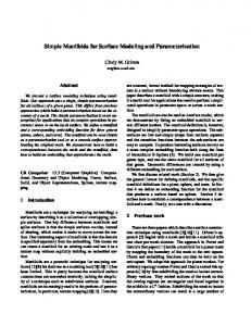
2 Historical Background The Greek astronomer Claudius Ptolemy (100–168 A.D.) was the first known to produce the data for creating a map showing the inhabited world as it was known to the Greeks and Romans of about 100–150 A.D. In his work Geography [89] he explains how to project a sphere onto a flat piece of paper using a system of gridlines—longitude and latitude. As we know from peeling oranges and trying to flatten the peels on a table, the sphere cannot be projected onto the plane without distortions and therefore certain compromises must be made. Fig. 1 shows some examples. The orthographic projection (a), which was known to the Egyptians and Greeks more than 2000 years ago, modifies both angles and areas, but the directions from the centre of projection are true. Probably the most widely used projection is the stereographic projection (b) usually attributed to Hipparchus (190–120 B.C.). It is a conformal projection, i.e., it preserves angles (at the expense of areas). It also maps circles to circles, no matter how large (great circles are mapped into straight lines), but a loxodrome is plotted as a spiral. A loxodrome is a line of constant bearing and of vital importance in navigation. In 1569, the Flemish cartographer Gerardus Mercator (1512–1594), whose goal was to produce a map which sailors could use to determine courses [87], overcame this drawback with his conformal cylindrical Mercator projection (c) which draws every loxodrome as a straight line. Neither the stereographic nor the Mercator projections preserve areas however. Johann Heinrich Lambert

(a)

(b)

(c)

(d)

Fig. 1. Orthographic (a), stereographic (b), Mercator (c), and Lambert (d) projection of the Earth.

Surface Parameterization

3

(1728–1777) found the first equiareal projection (d) in 1772 [86], at the cost of giving up the preservation of angles. All these projections can be seen as functions that map a part of the surface of the sphere to a planar domain and the inverse of this mapping is usually called a parameterization. Many of the principles of parametric surfaces and differential geometry were developed by Carl Friedrich Gauß (1777–1855), mostly in [81]. Conformal projections of general surfaces are of special interest due to their close connection to complex analytic functions, and the Riemann Mapping Theorem. This theorem, due to Bernhard Riemann (1826–1866) in his dissertation [91] of 1851, states that any simply-connected region of the complex plane can be mapped conformally into any other simply-connected region, such as the unit disk. It implies, similarly, that any disk-like surface can be mapped conformally into any simply-connected region of the plane.

3 Differential geometry background We take some basic theory of mappings from Kreyszig [85, Chap. VI]. Suppose a surface S ⊂ IR3 has the parametric representation x(u1 , u2 ) = (x1 (u1 , u2 ), x2 (u1 , u2 ), x3 (u1 , u2 )) for points (u1 , u2 ) in some domain in IR2 . We call such a representation regular if (i) the functions x1 , x2 , x3 are smooth, i.e., differentiable as many times as we need for our discussion, and (ii) the vectors x1 =

∂x , ∂u1

x2 =

∂x ∂u2

are linearly independent at every point (their cross product x1 × x2 is nonzero). Many properties of S are characterized by its first fundamental form, which is the square of the element of arc of a curve in S, the quadratic form 2

2

ds2 = x1 · x1 (du1 ) + 2 x1 · x2 du1 du2 + x2 · x2 (du2 ) . Writing gαβ = xα · xβ ,

α = 1, 2,

β = 1, 2,

and arranging the coefficients in a symmetric matrix µ ¶ g11 g12 I= g12 g22 we have

¶ du1 . ds = (du du ) I du2 2

1

2

µ

4

M. Floater and K. Hormann

f S

S¤

(u1,u2) = (u1¤,u2¤)

x

x¤

Fig. 2. The mapping f from S to S ∗ and the parameterization x of S induce the parameterization x∗ = f ◦ x of S ∗ .

Often, the matrix I is itself referred to as the first fundamental form. Under the assumption of regularity, this matrix has a strictly positive determinant 2 , g = det I = g11 g22 − g12

the discriminant of the quadratic form. In this case, the form is positive definite. The coefficients gαβ are the components of a covariant tensor of second order, called the metric tensor, denoted simply by gαβ . Suppose now that S is a surface with coordinates (u1 , u2 ) and that f is a mapping from S to a second surface S ∗ . Then we can define the parameterization x∗ = f ◦ x of S ∗ , so that the coordinates of any image point f (p) ∈ S ∗ are the same as those of the corresponding pre-image point p ∈ S; see Fig. 2. We say that the mapping f is allowable if the parameterization x∗ is regular. With this set up we will now consider various kinds of mappings. 3.1 Isometric mappings An allowable mapping from S to S ∗ is isometric or length-preserving if the length of any arc on S ∗ is the same as that of its pre-image on S. Such a mapping is called an isometry. For example, the mapping of a cylinder into the plane that transforms cylindrical coordinates into cartesian coordinates is isometric. Theorem 1. An allowable mapping from S to S ∗ is isometric if and only if the coefficients of the first fundamental forms are the same, i.e., I = I∗ .

Surface Parameterization

5

Two surfaces are said to be isometric if there exists an isometry between them. Isometric surfaces have the same Gaussian curvature at corresponding pairs of points (since Gaussian curvature depends only on the first fundamental form). 3.2 Conformal mappings An allowable mapping from S to S ∗ is conformal or angle-preserving if the angle of intersection of every pair of intersecting arcs on S ∗ is the same as that of the corresponding pre-images on S at the corresponding point. For example, the stereographic and Mercator projections are conformal maps from the sphere to the plane; see Fig. 1. Theorem 2. An allowable mapping from S to S ∗ is conformal or anglepreserving if and only if the coefficients of the first fundamental forms are proportional, i.e., I = η(u1 , u2 ) I∗ , (1) for some scalar function η 6= 0. 3.3 Equiareal mappings An allowable mapping from S to S ∗ is equiareal if every part of S is mapped onto a part of S ∗ with the same area. For example, the Lambert projection is an equiareal mapping from the sphere to the plane; see Fig. 1. Theorem 3. An allowable mapping from S to S ∗ is equiareal if and only if the discriminants of the first fundamental forms are equal, i.e., g = g∗.

(2)

The proofs of the above three results can be found in Kreyszig [85]. It is then quite easy to see the following (see also Kreyszig): Theorem 4. Every isometric mapping is conformal and equiareal, and every conformal and equiareal mapping is isometric, i.e., isometric ⇔ conformal + equiareal. We can thus view an isometric mapping as ideal, in the sense that it preserves just about everything we could ask for: angles, areas, and lengths. However, as is well known, isometric mappings only exist in very special cases. When mapping into the plane, the surface S would have to be developable, such as a cylinder. Many approaches to surface parameterization therefore attempt to find a mapping which either 1. is conformal, i.e., has no distortion in angles, or 2. is equiareal, i.e., has no distortion in areas, or 3. minimizes some combination of angle distortion and area distortion.

6

M. Floater and K. Hormann

3.4 Planar mappings A special type of mappings that we will consider now and then in the following are planar mappings f : IR2 → IR2 , f (x, y) = (u(x, y), v(x, y)). For these kind of mappings the first fundamental form can be written as I = J TJ ¢ ¡ where J = uvxx uvyy is the Jacobian of f . It follows that the singular values σ1 and σ2 of J are just the square roots of the eigenvalues λ1 and λ2 of I and it is then easy to verify Proposition 1. For a planar mapping f : IR2 → IR2 the following equivalencies hold: ¡ ¢ 1. f is isometric ⇔ I = 10 01 ⇔ λ1 = λ2 = 1 ⇔ σ1 = σ2 = 1, ¡η 0¢ ⇔ λ1 /λ2 = 1 ⇔ σ1 /σ2 = 1, 2. f is conformal ⇔ I = 0 η 3.

f is equiareal

⇔

det I = 1

⇔

λ 1 λ2 = 1

⇔

σ1 σ2 = 1.

4 Conformal and harmonic mappings Conformal mappings have many nice properties, not least of which is their connection to complex function theory. Consider for the moment the case of mappings from a planar region S to the plane. Such a mapping can be viewed as a function of a complex variable, ω = f (z). Locally, a conformal map is simply any function f which is analytic in a neighbourhood of a point z and such that f 0 (z) 6= 0. A conformal mapping f thus satisfies the CauchyRiemann equations, which, with z = x + iy and ω = u + iv, are ∂v ∂u = , ∂x ∂y

∂u ∂v =− . ∂y ∂x

(3)

Now notice that by differentiating one of these equations with respect to x and the other with respect to y, we obtain the two Laplace equations ∆u = 0, where ∆=

∆v = 0,

∂2 ∂2 + ∂x2 ∂y 2

is the Laplace operator. Any mapping (u(x, y), v(x, y)) which satisfies these two Laplace equations is called a harmonic mapping. Thus a conformal mapping is also harmonic, and we have the implications isometric ⇒ conformal ⇒ harmonic.

Surface Parameterization

7

f S

S¤

Fig. 3. One-to-one harmonic mappings.

Why do we consider harmonic maps? Well, their big advantage over conformal maps is the ease with which they can be computed, at least approximately. After choosing a suitable boundary mapping (which is equivalent to using a Dirichlet boundary condition for both u and v), each of the functions u and v is the solution to a linear elliptic partial differential equation (PDE) which can be approximated by various methods, such as finite elements or finite differences, both of which lead to a linear system of equations. Harmonic maps are also guaranteed to be one-to-one for convex regions. The following result was conjectured by Rad´o [90] and proved independently by Kneser [84] and Choquet [80]. Theorem 5 (RKC). If f : S → IR2 is harmonic and maps the boundary ∂S homeomorphically into the boundary ∂S ∗ of some convex region S ∗ ⊂ IR2 , then f is one-to-one; see Fig. 3. On the downside, harmonic maps are not in general conformal and do not preserve angles. For example, it is easy to verify from the Cauchy-Riemann 2 and Laplace equations that the bilinear mapping f : [0, 1] → IR2 defined by u = x(1 + y),

v = y,

is harmonic but not conformal. Indeed the figure below clearly shows that this harmonic map does not preserve angles.

f

Fig. 4. A harmonic mapping which is not conformal.

Another weakness of harmonic mappings is their “one-sidedness”. The inverse of a harmonic mapping is not necessarily harmonic. Again, the bilinear example above provides an example of this. It is easy to check that the inverse

8

M. Floater and K. Hormann

mapping x = u/(1 + v), y = v is not harmonic as the function x(u, v) does not satisfy the Laplace equation. Despite these drawbacks, harmonic mappings do at least minimize deformation in the sense that they minimize the Dirichlet energy Z Z ¡ 1 1 2 2¢ 2 ED (f ) = k∇uk + k∇vk . kgradf k = 2 S 2 S

This property combined with their ease of computation explains their popularity. When we consider mappings from a general surface S ⊂ IR3 to the plane, we find that all the above properties of conformal and harmonic mappings are essentially the same. The equations just become more complicated. Any mapping f from a given surface S to the plane defines coordinates of S, say (u1 , u2 ). By Theorem 2, if f is conformal then there is some scalar function η 6= 0 such that ¡ 2 2¢ ds2 = η(u1 , u2 ) (du1 ) + (du2 ) . Suppose that S has given coordinates (˜ u1 , u ˜2 ). After some analysis (see Chap. VI of Kreyszig), one can show that the above equation implies the two equations g˜11 ∂u2 g˜12 ∂u2 ∂u1 √ √ = − , ∂u ˜1 ˜2 ˜1 g˜ ∂ u g˜ ∂ u

∂u1 −˜ g22 ∂u2 g˜12 ∂u2 √ √ = + , ∂u ˜2 ˜1 ˜2 g˜ ∂ u g˜ ∂ u

(4)

which are a generalization of the Cauchy-Riemann equations (3). Indeed, in the special case that S is planar, we can take g˜11 = g˜22 = 1,

g˜12 = 0,

(5)

and we get simply

∂u1 ∂u2 ∂u1 ∂u2 = , = − 1. 1 2 2 ∂u ˜ ∂u ˜ ∂u ˜ ∂u ˜ Similar to the planar case, we can differentiate one equation in (4) with respect to u ˜1 and the other with respect to u ˜2 , and obtain the two generalizations of Laplace’s equation, ∆S u1 = 0, ∆S u2 = 0, (6) where ∆S is the Laplace-Beltrami operator µ µ ¶ µ ¶¶ 1 g˜12 ∂ g˜12 ∂ ∂ g˜22 ∂ ∂ g˜11 ∂ √ √ ∆S = √ −√ −√ + . ˜1 ˜1 ˜2 ∂u ˜2 ˜2 ˜1 g˜ ∂ u g˜ ∂ u g˜ ∂ u g˜ ∂ u g˜ ∂ u When this operator is differentiated out, one finds that it is a linear elliptic operator with respect to the coordinates (˜ u1 , u ˜2 ) (as noted and exploited by Greiner [82]). The operator generalizes the Laplace operator (as can easily be checked by taking S to be planar with g˜αβ as in (5)), and is independent of the

Surface Parameterization

9

particular coordinates (in this case (˜ u1 , u ˜2 )) used to define it. As explained by Klingenberg [83], it can also be written simply as ∆S = divS gradS . Similar to the planar case, a harmonic map can either be viewed as the solution to equation (6), or as the minimizer of the Dirichlet energy Z 1 2 kgradS f k ED (f ) = 2 S over the surface S.

5 Equiareal mappings As we saw in Sec. 3, there are essentially only two quantities to consider minimizing in a mapping: angle distortion and area distortion. We know from the Riemann mapping theorem that (surjective) conformal mappings from a disk-like surface to a fixed planar simply-connected region not only exist but are also almost unique. For example, consider mapping the unit disk S into itself (treating S as a subset of the complex plane), and choose any point z ∈ S and any angle θ, −π < θ ≤ π. According to the theorem, there is precisely one conformal mapping f : S → S such that f (z) = 0 and arg f 0 (z) = θ. In this sense there are only the three degrees of freedom defined by the complex number z and the real angle θ in choosing the conformal map. What we want to do now is to demonstrate that equiareal mappings are substantially different to conformal ones from the point of view of uniqueness as there are many more of them. The following example is to our knowledge novel and nicely illustrates the abundance of equiareal mappings. Consider again mappings f : S → S, from the unit disk S into itself. Using the polar coordinates x = r cos θ, y = r sin θ, one easily finds that the determinant of the Jacobian of any mapping f (x, y) = (u(x, y), v(x, y)) can be expressed as det J(f ) = ux vy − uy vx =

1 (ur vθ − uθ vr ). r

Consider then the mapping f : S → S defined by ¡ ¢ r(cos θ, sin θ) 7→ r cos(θ + φ(r)), sin(θ + φ(r)) ,

for 0 ≤ r ≤ 1 and −π < θ ≤ π, where φ : [0, 1] → IR is an arbitrary function. This mapping maps each circle of radius r centred at the origin into itself, rotated by the angle φ(r); see Fig. 5. If φ is differentiable then so is f and differentiation shows that ur vθ − uθ vr = r,

10

M. Floater and K. Hormann

f

Fig. 5. An equiareal mapping.

independent of the function φ. We conclude that det J(f ) = 1 and therefore, according to Proposition 1, f is equiareal, irrespective of the chosen univariate function φ. It is not difficult to envisage other families of equiareal mappings constructed by rotating circles about other centres in S. These families could also be combined to make further equiareal mappings. When we consider again the formulations of conformal and equiareal mappings in terms of the first fundamental form, the lack of uniqueness of equiareal mappings becomes less surprising. For, as we saw earlier, the property of conformality (1) essentially places two conditions on the three coefficients of the ∗ ∗ ∗ first fundamental form g11 , g12 , g22 , while the property of equiarealness (2) places only one condition on them (the three conditions together of course completely determine the three coefficients, giving an isometric mapping). Considering not only the non-uniqueness, but also the rather strange rotational behaviour of the above mappings, we conclude that it is hardly sensible to try to minimize area deformation alone. In order to find a well-behaved mapping we surely need to combine area-preservation with some minimization of angular distortion.

6 Discrete harmonic mappings Common to almost all surface parameterization methods is to approximate the underlying smooth surface S by a piecewise linear surface ST , in the form of a triangular mesh, i.e. the union of a set T = {T1 , . . . , TM } of triangles Ti such that the triangles intersect only at common vertices or edges. Nowadays in fact, surfaces are frequently simply represented as triangular meshes, and the smooth underlying surface is often not available. We will denote by V the set of vertices. If ST has a boundary, then the boundary will be polygonal and we denote by VB the set of vertices lying on the boundary and by VI the set of interior vertices. The most important parameterization task is to map a given disk-like surface S ⊂ IR3 into the plane. Working with a triangular mesh ST , the goal is to find a suitable (polygonal) domain S ∗ ⊂ IR2 and a suitable piecewise linear mapping f : ST → S ∗ that is linear on each triangle Ti in ST and continuous; see Fig. 6. Such a mapping is uniquely determined by the images f (v) ∈ IR2 of the vertices v ∈ V .

Surface Parameterization

11

f S¤

ST

Fig. 6. Piecewise linear mapping of a triangular mesh.

6.1 Finite element method One of the earliest methods for mapping disk-like surfaces into the plane was to approximate a harmonic map using the finite element method based on linear elements. This method was introduced to the computer graphics community by Eck et al. [12] and called simply a discrete harmonic map, although a similar technique had earlier been used by Pinkall and Polthier for computing piecewise linear minimal surfaces [56]. The basic method has two steps. 1. First fix the boundary mapping, i.e. fix f |∂ST = f0 , by mapping the polygonal boundary ∂ST homeomorphically to some polygon in the plane. This is equivalent to choosing the planar image of each vertex in the mesh boundary ∂ST and can be done in several ways (see [14] or [33, Sec. 1.2.5] for details). 2. Find the piecewise linear mapping f : ST → S ∗ which minimizes the Dirichlet energy Z 1 2 ED = kgradST f k , 2 ST subject to the Dirichlet boundary condition f |∂ST = f0 . The main advantage of this method over earlier approaches is that this is a quadratic minimization problem and reduces to solving a linear system of equations. Consider one triangle T = [v1 , v2 , v3 ] in the surface ST . Referring to Fig. 7, one can show that Z 2 2 kgradT f k = cot θ3 kf (v1 ) − f (v2 )k 2 T

2

2

+ cot θ2 kf (v1 ) − f (v3 )k + cot θ1 kf (v2 ) − f (v3 )k .

The normal equations for the minimization problem can therefore be expressed as the linear system of equations

12

M. Floater and K. Hormann

v3

v1 µ1

f(v3)

fjT

µ3

®3

T

f(T) ®2 ®1

µ2

f(v2)

f(v1)

v2

Fig. 7. Atomic map between a mesh triangle and the corresponding parameter triangle.

X

j∈Ni

wij (f (vj ) − f (vi )) = 0,

v i ∈ VI ,

(7)

where wij = cot αij + cot βij

(8)

and the angles αij and βij are shown in the figure below. Here we have assumed that the vertices in V are indexed (in any random order) and that Ni denotes the set of indexes of the neighbours of the vertex vi (those vertices which share an edge with vi ).

vj

®ij ±ij °ij

¯ij

vi Fig. 8. Angles for the discrete harmonic map and the mean value coordinates.

The associated matrix is symmetric and positive definite, and so the linear system is uniquely solvable. The matrix is also sparse and iterative methods are effective, e.g., conjugate gradients. Note that the system has to be solved twice, once for the x- and once for the y-coordinates of the parameter points f (vi ), vi ∈ VI . In practice the method often gives good visual results. 6.2 Convex combination maps The theory of finite elements [79] provides a well-established convergence theory for finite element approximations to second order elliptic PDE’s. Extrap-

Surface Parameterization

13

olating this theory, we can argue that the error incurred when discretizing a harmonic map f : S → S ∗ , S ∗ ⊂ IR2 , from a smooth surface to the plane, by a discrete harmonic map over some triangular mesh ST of S, will tend to zero as the mesh size tends to zero (in an appropriate norm and under certain conditions on the angles of the triangles). Due to the RKC Theorem 5, it is therefore reasonable to expect that, with S ∗ convex, a discrete harmonic map f : ST → S ∗ , like its harmonic cousin, will be one-to-one, i.e., that for every oriented triangle T = [v1 , v2 , v3 ] in the surface ST , the mapped triangle f (T ) = [f (v1 ), f (v2 ), f (v3 )] would be nondegenerate and have the same orientation. It turns out that this is guaranteed to be true if all the weights wij in Equation (7) are positive. To understand this, note that if we define the normalized weights . X λij = wij wik , k∈Ni

for each interior vertex vi , we can re-express the system (7) as X f (vi ) = λij f (vj ), vi ∈ V I .

(9)

j∈Ni

It follows that if all the weights wij are positive then so are the weights λij and the piecewise linear mapping f demands that each mapped interior vertex f (vi ) will be a convex combination of its neighbours f (vj ), and so must lie in their convex hull. It is reasonable to call any piecewise linear mapping of this kind a convex combination mapping. The special case in which the weights λ ij are uniform, i.e., for each interior vertex vi they are equal to 1/di , where di is the valency of vertex vi , was called a barycentric mapping by Tutte [92] (in a more abstract graph-theoretic setting). Each image point f (vi ) is forced to be the barycentre of its neighbours. Tutte showed the following. Theorem 6 (Tutte). A barycentric mapping of any simple 3-connected planar graph G is a valid straight line embedding. It was later observed in [14] that this theorem applies to triangular meshes, and moreover, that Tutte’s proof could be extended in a simple way to allow P arbitrary positive weights λij in Equation (9) satisfying j∈Ni λij = 1. Recently, an independent and simpler proof of this result was given in [19]: Theorem 7. If f : ST → S ∗ is a convex combination mapping which maps ∂ST homeomorphically into a convex polygon ∂S ∗ , then f is one-to-one. Recalling the weights of Equation (8), notice from trigonometry that cot αij + cot βij =

sin(αij + βij ) , sin αij sin βij

and so wij > 0

⇐⇒

Therefore, it follows (see again [19]):

αij + βij < π.

14

M. Floater and K. Hormann

Proposition 2. A discrete harmonic map f : ST → S ∗ is one-to-one if it maps ∂ST homeomorphically into a convex polygon ∂S ∗ and if the sum of every pair of opposite angles of quadrilaterals in ST is less than π. Generally speaking, this opposite-angle condition is fulfilled when the triangles are “well-shaped”, and holds in particular when all angles of all triangles in ST are less than π/2. Conversely, counterexamples have been constructed (a numerical one in Duchamp et al. [11] and an analytical one in [15]) which show that if the opposite-angle condition does not hold then the discrete harmonic map may not be one-to-one: some triangles “flip over”, i.e. have the wrong orientation. We envisage two possible ways of tackling this problem. The first approach is to perform some preprocessing operation on the given triangular mesh and insert new vertices to split triangles and perhaps swap some edges in order to obtain a new mesh for which the opposite angle condition holds. Of course, if the mesh is planar, we could simply use the well-known Delaunay swap criterion, and we would eventually end up with a Delaunay triangulation, which certainly satisfies the opposite angle condition in every quadrilateral. However, we do not know of any concrete swapping procedure in the literature which provides the same guarantee for a general surface mesh. The other alternative is to design a convex combination map with good properties and if possible to mimic the behaviour of a harmonic map. 6.3 Mean value coordinates In addition to injectivity, another natural property that we can expect from a mapping is to be an isometry whenever possible. It is well-known [83, 85] that such an isometry exists if and only if the surface S is developable. Piecewise linear surfaces ST are developable if the angles around each interior vertex sum up to 2π which rarely is the case, unless ST is planar. We therefore propose that a good piecewise linear mapping should have the following reproduction property: In the case that the surface mesh ST is planar and its planar polygonal boundary is mapped affinely into the plane, then the whole mapping should be the same affine mapping. Discrete harmonic maps have this reproduction property but are not guaranteed to be injective. The shape-preserving method of [14] is a convex combination mapping (and therefore always one-to-one for convex images), designed also to have this reproduction property. In many numerical examples, the discrete harmonic map and shape-preserving maps look visually very similar, especially when the surface is not far from planar. For more complex shapes, the two methods begin to differ more, with the shape-preserving map being more robust in the presence of long and thin triangles. A more recent paper [18] gives an alternative construction of a convex combination mapping with the reproduction property, which both simplifies the shape-preserving method of [14] and at the same time directly discretizes

Surface Parameterization

(a)

(b)

(c)

(d)

15

(e)

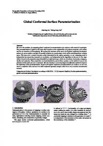
Fig. 9. Remeshing a triangle mesh with a regular quadrilateral mesh using different parameterization methods.

a harmonic map. It is based on mean value coordinates and motivated as explained below. The numerical results are quite similar to the shape-preserving parameterization. Fig. 9 shows the result of first mapping a triangle mesh (a) to a square and then mapping a regular rectangular grid back onto the mesh. The four mappings used are barycentric (b), discrete harmonic (c), shape-preserving (d), and mean value (e). The idea in [18] is the observation that harmonic functions (and therefore also harmonic maps) satisfy the mean value theorem. At every point in its (planar) domain, the value of a harmonic function is equal to the average of its values around any circle centred at that point. This suggests finding a piecewise linear map f : ST → S ∗ , for a planar triangular mesh ST , which satisfies the mean value theorem at every interior vertex vi of the mesh. We let Γi be a circle centred at vi with radius ri > 0 small enough that Γi only intersects triangles in T which are incident on vi . We then demand that Z 1 f (v) ds. f (vi ) = 2πri Γi Some algebra then shows that independent of ri > 0 (for ri small enough), the above equation is the same as Equation (7) but with the weights wij replaced by tan(δij /2) + tan(γij /2) , wij = ||vj − vi || with the angles shown in Fig. 8. When ST is a surface mesh, we simply use the same weights with the angles δij and γij taken from the mesh triangles. For a recent in-depth comparison of computational aspects of discrete harmonic maps and mean value maps, including multilevel solvers, see Aksoylu, Khodakovsky, and Schr¨oder [1]. Energy minimization We have seen that mean value maps discretize harmonic maps in a certain way, but in contrast to discrete harmonic maps they are not the solution

16

M. Floater and K. Hormann

of a minimization problem. This makes them a bit special because all other parameterization methods in the literature stem from the minimization of some energy. For example, discrete harmonic maps minimize the Dirichlet energy, and recently Guskov [29] showed that the shape-preserving maps minimize an energy that is based on second differences. But these are not the only energies that are minimized by convex combination maps. Greiner and Hormann [25] showed that any choice of symmetric weights wij = wji in (7) minimizes a spring energy and Desbrun, Meyer, and Alliez [10] proposed the chi energy that is minimized if the Wachspress coordinates [93, 94, 88] are taken as w ij . An interesting question for future research is if there also exists a meaningful energy that is minimized by mean value mappings. 6.4 The boundary mapping The first step in constructing both the discrete harmonic and the convex combination maps is to choose the boundary mapping f |∂ST . There are two issues here: (i) choosing the shape of the boundary, and (ii) choosing the distribution of the points around the boundary. Choosing the shape In many applications, it is sufficient (or even desirable) to map to a rectangle or a triangle, or even a polygonal approximation to a circle. In all these cases, the boundary is convex and the methods of the previous section work well. The convexity restriction may, however, generate big distortions near the boundary when the boundary of the surface ST does not resemble a convex shape. One practical solution to avoid such distortions is to build a “virtual” boundary, i.e., to augment the given mesh with extra triangles around the boundary so as to construct an extended mesh with a “nice” boundary. This approach has been successfully used by Lee, Kim, and Lee [43], and K´os and V´arady [40]. Choosing the distribution Consider first the case of a smooth surface S with a smooth boundary ∂S. Due to the Riemann Mapping Theorem we know that S can be mapped into any given simply-connected region S ∗ ⊂ IR2 by a conformal map f : S → S ∗ . Since any such conformal map defines a boundary mapping f |∂S : ∂S → ∂S ∗ , this implies (assuming smooth well-behaved boundaries) that there must exist some boundary mapping such that the harmonic map it defines is also conformal. Such a boundary mapping seems like an ideal mapping to aim for. However, to the best of our knowledge it is not known how to find one. Thus in the case of piecewise linear mappings, the usual procedure in the literature is to choose some simple boundary mapping such as chord length

Surface Parameterization

17

parameterization (for polygons), either around the whole boundary, or along each side of the boundary when working with triangular or rectangular boundaries. An interesting topic for future research is to search for better ways to distribute the mapped boundary points around a fixed, chosen boundary (such as a circle). It seems likely that finding a distribution that maximizes the conformality of the whole mapping will depend at least on the global shape of the surface mesh boundary and perhaps on the shape of the surface itself. As far as we know this issue has not yet been addressed in the literature.

7 Discrete conformal mappings In all the parameterization methods described in the previous section, the boundary mapping f |∂ST had to be fixed in advance and preferably map to a convex polygon. There are, however, several approaches that maximize the conformality of the piecewise linear mapping without demanding the mesh boundary to be mapped onto a fixed shape. Instead, these methods allow the parameter values of the boundary points to be included into the optimization problem and the shape of the parameter domain is determined by the method. 7.1 Most isometric parameterizations The method of Hormann and Greiner [34] is based on measuring the conformality of a (non-degenerate) bivariate linear function g : IR2 → IR2 by the condition number of its Jacobian J with respect to the Frobenius-norm, which can be expressed in terms of the singular values σ1 and σ2 of J as follows: q q σ2 σ1 + . EM (g) = κF (J) = kJkF kJ −1 kF = σ12 + σ22 1/σ12 + 1/σ22 = σ2 σ1

According to Proposition 1 this functional clearly is minimal if and only if g is conformal. Since each atomic map f |T : T → IR2 can be seen as such a bivariate linear function, the conformality of the piecewise linear mapping f is then defined as X EM (f |T ). (10) EM (f ) = T ∈T

This energy is bounded from below by twice the number of triangles in T and this minimum is obtained if and only if f is conformal. Thus, minimizing (10) gives a parameterization that is as conformal as possible. Note that piecewise linear functions can only be conformal if the surface ST is developable and conformality implies isometry in this case. Hence the term “most isometric parameterizations” (MIPS). Interestingly, the notion of singular values is also useful to express the Dirichlet energy of a linear mapping g(x, y) = (u(x, y), v(x, y)). Using the identity

18

M. Floater and K. Hormann

σ12 + σ22 = trace (J TJ) = trace (I) = u2x + u2y + vx2 + vy2

(11)

we find for any planar region S that Z Z 1 1 1 2 2 2 ED (g) = kgrad gk = (k∇uk + k∇vk ) = (σ12 + σ22 )A(S), 2 S 2 S 2 where A(S) denotes the area of S. Further considering the identity σ1 σ2 = det J = ux vy − uy vx = A(g(S))/A(S)

(12)

reveals a close relation between the MIPS energy of an atomic map and its Dirichlet energy, ED (f |T ) . EM (f |T ) = 2 A(f (T )) This underlines the conformality property of the MIPS method since it is well known that ED (f |T ) ≥ A(f (T )) with equality if and only if f is conformal. It also shows that the MIPS energy in (10) is a sum of quadratic rational functions in the unknown parameter values f (v) and thus the minimization is a non-linear problem. As proposed in [36], this problem can be solved in the following way. Starting from an initial barycentric mapping, each planar vertex is repeatedly relocated in order to minimize the functional locally there. During this iteration, each vertex pi = f (vi ) in the current planar mesh lies in the kernel Ki of the star-shaped polygon formed by its neighbours. Since the MIPS energy is infinite if any mapped triangle f (T ) is degenerate, it is infinite on the boundary of the kernel Ki . There must therefore be a local minimum to the local functional somewhere in the interior of Ki . In fact, it has been shown in [33, Sec. 1.3.2] that the local functional is convex over the interior of Ki and that the local minimum can be found efficiently using Newton’s method. By moving pi to this minimum, the method ensures that the updated planar mesh will not have any folded triangles. 7.2 Angle-based flattening While the conformality condition used in the previous section is trianglebased and can be expressed in terms of the parameter values f (v), v ∈ V , the method of Sheffer and de Sturler [69] minimizes a pointwise criterion that is formulated in terms of the angles of the parameter triangles. Let us denote by θi the mesh angles in ST and by αi the corresponding planar angles in S ∗ We further define I(v) as the set of indices Pof the angles around a vertex v ∈ V and the sum of these angles, θ(v) = i∈I(v) θi . For any interior vertex v ∈ VI , the planar angles αi , i ∈ I(v) sum up to 2π, but the corresponding mesh angles usually do not. This angular deformation is inevitable for piecewise linear mappings and the best one can hope for is that the deformation is distributed evenly around the vertex. Sheffer and de Sturler

Surface Parameterization

19

therefore define for each v ∈ V the optimal angles βi = θi s(v), i ∈ I(v) with a uniform scale factor ½ 2π/θ(v), v ∈ VI , s(v) = 1, v ∈ VB , and determine an optimal set of planar angles by minimizing the energy X 2 E(α) = (αi /βi − 1) . (13) i

They finally construct the parameter values f (v) and thus the piecewise linear mapping f itself from the angles αi . Though the minimization problem is linear in the unknowns αi , it becomes non-linear as a number of constraints (some of which are non-linear) have to be taken into account to guarantee the validity of the solution. A simplification of these constraints as well as a discussion of suitable solvers can be found in [77]. Like in the previous section, the energy in (13) is bounded from below and the minimum is obtained if and only if ST is developable with θ(v) = 2π at all interior vertices and f is conformal with αi = βi = θi for all i. 7.3 Linear methods L´evy et al. [47] and Desbrun et al. [10] both independently developed a third method to compute discrete conformal mappings which has the advantage of being linear. For a bivariate linear function g : IR2 → IR2 , L´evy et al. propose measuring the violation of the Cauchy-Riemann equations (3) in a least squares sense, i.e., with the conformal energy EC (g) =

1¡ 2 2¢ (ux − vy ) + (uy + vx ) . 2

Based on this they find the optimal piecewise linear mapping f : ST → S ∗ by minimizing X EC (f ) = EC (f |T )A(T ). T ∈T

Like the MIPS energy, EC (g) can be expressed in terms of the singular values of the Jacobian of g and there is a close relation to the Dirichlet energy. Using (11) and (12) we find 1 2 EC (g) = (σ1 − σ2 ) 2 and EC (g)A(S) = ED (g) − A(g(S)) for any planar region S. Therefore we have EC (f ) = ED (f ) − A(f ),

20

M. Floater and K. Hormann

which also shows that EC (f ) is quadratic in the unknowns f (v) and that the normal equations for the minimization problem can therefore be expressed as a linear system of equations. Desbrun et al. take a slightly different path to arrive at the same system. They start with the finite element method (see Sec. 6.1) that yields the equations Dp ED (f ) = 0 for all parameter points p = f (v) of the interior vertices v ∈ VI ; compare (7). But instead of fixing the boundary f |∂ST , they impose natural boundary constraints, Dp ED (f ) = Dp A(f ), for all p = f (v), v ∈ VB . But as they also show that Dp A(f ) = 0 at the interior vertices, this amounts to solving grad ED = grad A, and is thus equivalent to minimizing EC (f ). However, as EC (f ) is clearly minimized by all degenerate mappings f that map ST to a single point, additional constraints are needed to find a unique and non-trivial solution. Both papers therefore propose to fix the parameter values f (v), f (w) of two vertices v, w ∈ V . The solution depends on this choice. For example, if we parameterize the pyramid in Fig. 10 (a) whose vertices lie on the corners of a cube, fixing p1 = f (v1 ) and p2 = f (v2 ) gives the solution in (b), while fixing p1 = f (v1 ) and p3 = f (v3 ) results in the parameterization shown in (c).

v5 p4

p4

p3

p3

v3

v4

p5 p1 v1

p2

v2 (a)

(b)

p5 p1

p2 (c)

Fig. 10. Example of two different discrete conformal mappings for the same triangulation.

Note that the x- and y-coordinates of the parameter points f (v) are coupled in this approach since the areas of the parameter triangles are involved. Thus the size of the system to be solved is roughly twice as large as the one for discrete harmonic maps (see Sec. 6.1). We further remark that unlike the MIPS and the angle based flattening methods, this approach may generate folded triangles and that we do not know

Surface Parameterization

21

of any sufficient conditions that guarantee the resulting parameterization to be a one-to-one mapping.

8 Discrete equiareal mappings In view of the high degree of non-uniqueness of equiareal mappings shown in Sec. 5, it is not surprising that discrete (piecewise linear) equiareal mappings are also far from unique and also exhibit strange behaviour. For example, an obvious attempt at an area-preserving mapping f : ST → S ∗ , S ∗ ⊂ IR2 , for a triangular mesh ST ⊂ IR3 is to fix the polygonal region S ∗ to have the same area as that of ST , and then to find f which minimizes a functional like X¡ ¢2 A(f (T )) − A(T ) . E(f ) = T ∈T

Unlike the discrete Dirichlet energy, this functional is no longer quadratic in the coordinates of the image points f (v). Not surprisingly, there exist meshes for which E has several minima, and moreover several mappings f such that E(f ) = 0. Fig. 11 shows an example in which the area A(f (T )) of each image triangle is equal to the area of the corresponding domain triangle A(T ) and thus E(f ) = 0. In other words, f is a (discrete) equiareal mapping.

Fig. 11. Two planar meshes whose corresponding triangles have the same area.

Other examples of minimizing the functional E and its variants often produce long and thin triangles. In some cases triangles flip over. Maillot, Yahia, and Verroust [52] gave a variant of E in which each term in the sum is divided by A(T ), but few numerical examples are given in their paper. Surazhsky and Gotsman [76] have found area-equilization useful for other purposes, specifically for remeshing. Recently, Degener et al. [9] extended the MIPS method to find parameterizations that mediate between angle and area deformation. They measure the area deformation of a bivariate linear function g by EA (g) = det J +

1 1 = σ 1 σ2 + , det J σ1 σ2

22

M. Floater and K. Hormann

which, according to Proposition 1, clearly is minimal if and only if g is equiareal. They then minimize the overall energy X q EM (f |T )EA (f |T ) A(T ), E(f ) = T ∈T

where q ≥ 0 is a parameter that controls the relative importance of the angle and the area deformation. Note that the case q = 0 corresponds to minimizing angle deformation alone, but that no value of q gives pure minimization of areas. Sander et al. [62] explore methods based on minimizing functionals that measure the “stretch” of a mapping. These appear to retain some degree of conformality in addition to reducing area distortion and seem to perform well in numerical examples. In the notation of Sec. 7.1 they measure the stretch of a bivariate linear mapping g : IR2 → IR2 by q E2 (g) = kJkF = σ12 + σ22 and E∞ (g) = kJk∞ = σ1 and minimize one of the two functionals v uP 2 u A(T )E2 (f |−1 T ) E2 (f ) = t T ∈TP , T ∈T A(T )

E∞ (f ) = max E∞ (f |−1 T ). T ∈T

Note that both functionals accumulate the stretch of the inverse atomic maps f |−1 T that map from the parameter to the surface triangle. Sander et al. minimize these non-quadratic functionals with an iterative method similar to the one described in Sec. 7.1. Like the MIPS method, both stretch functionals always yield a one-to-one mapping. Numerical examples showing comparisons with discrete harmonic maps are given in [62].

9 Parameterization methods for closed surfaces 9.1 Surfaces with genus zero There has been a lot of interest in spherical parameterization recently and in this section we will briefly summarize recent work. Many of the methods attempt to mimic conformal (or harmonic) maps and are very similar to those for mapping disk-like surfaces into the plane, although some of the linear methods now become non-linear. An important point is that, according to Gu and Yau [27], harmonic maps from a closed genus zero surface to the unit sphere are conformal, i.e., harmonic and conformal maps are the same when we deal with (closed) sphere-like surfaces. Intuitively, this follows from the fact that the domain and image have no boundary, and it is exactly the boundary map that makes the difference

Surface Parameterization

23

between a conformal and a harmonic map in the planar case. According to Gu and Yau there are essentially only six “degrees of freedom” (the M¨obius transformations) in a spherical conformal map, three of which are rotations, the others involving some kind of area distortion (angles are of course preserved by definition). The method of Haker et al. [32] first maps the given sphere-like surface ST into the plane and then uses stereographic projection (itself a conformal map) to subsequently map to the sphere. The planar mapping part of this construction appears to reduce to the usual discrete harmonic map described in Sec. 6.1. Unfortunately, it is not clear in [32] how the surface is split or cut to allow for a mapping into the plane and how the boundary condition is treated. Gu and Yau [28] have later proposed an iterative method which approximates a harmonic (and therefore conformal) map and avoids splitting. Specifically, a harmonic map from a closed surface S to the unit sphere S ∗ is a map f : S → S ∗ such that at every point p of S, the vector ∆S f (p) ∈ IR3 is perpendicular to the tangent plane of S ∗ at f (p). In the discrete case we consider piecewise linear mappings f : ST → IR3 over an approximative mesh ST with the property that f (v) lies on the unit sphere S ∗ for every vertex v ∈ V of the mesh ST . Gu and Yau propose approximating a harmonic (conformal) map in the following way. Let Πvi (u) denote the perpendicular projection of any point u on the sphere S ∗ onto the tangent plane of S ∗ at vi . Then they consider a map which solves the (non-linear) equations X ¡ ¢ wij Πvi (f (vj )) − f (vi ) = 0, vi ∈ V, j∈Ni

where, as in the planar case (7), the coefficients wij are the weights of (8). Gu and Yau [28] give many nice numerical examples based on their method. However, numerical difficulties apparently arise when some of the weights w ij are negative, and they propose editing the original surface mesh, so that all weights are positive, though no procedure for doing this is given. One might expect that a piecewise linear map should be one-to-one if all the weights are positive. Gotsman, Gu, and Sheffer have dealt with this issue in [24]. They work with the alternative equations X wij f (vj ) = λi f (vi ), vi ∈ V. j∈Ni

This equation says that a certain (positive) linear combination of the neighbouring vectors f (vj ) must be parallel to the unit vector f (vi ), and the factor λi > 1 is to be determined. Such a mapping is a spherical barycentric (or convex combination) mapping. When the weights wij are constant with respect to j we get an analogue of Tutte’s barycentric mapping into the plane. A theorem by Colin de Verdi`ere, described in [24], guarantees a valid embedding into the sphere if certain conditions on the eigenvalues of the matrix formed by the

24

M. Floater and K. Hormann

left hand sides of the equation hold. Unfortunately, it is currently not known how to guarantee these conditions and examples of simple meshes can be constructed for which there are several possible barycentric mappings, some of which are not one-to-one. However, the paper by Gotsman, Gu, and Sheffer looks like a good start-point for future work in this direction. The angle-based method of Sheffer and de Sturler [69] has been generalized in a straightforward manner to the spherical case by Sheffer, Gotsman, and Dyn [71] using a combination of angle and area distortion. The stretch metric approach of Sander et al. [62] has been generalized to the spherical case by Praun and Hoppe [58]. 9.2 Surfaces with arbitrary genus A well-known approach to parameterizing (mesh) surfaces of arbitrary genus over simpler surfaces of the same genus is to somehow segment the mesh into disk-like patches and then map each patch into the plane. Usually, triangularshaped patches are constructed and each patch is mapped to a triangle of a so-called base mesh. The challenge of this approach is to obtain mappings that are smooth across the patch boundaries and the first methods [12, 42, 59, 30, 21] suffered indeed from this problem. But recently Khodakovsky, Litke, and Schr¨oder [38] and Gu and Yau [28] proposed two different methods to compute parameterizations that are globally smooth with singularities occurring at only a few extraordinary vertices.

10 Conclusion We have summarized as best we can both early and recent advances in the topic of surface parameterization. In addition to the 35 papers we have mentioned earlier in the text, we have added to the reference list a further 43 references to papers on surface parameterization, giving a total of 78 papers. We feel it fair to say that the topic, as we know it now, began with the 1995 paper on the discrete harmonic map by Eck et al. [12], though essentially the same method was proposed in 1993 by Pinkall and Polthier [56] for computing minimal surfaces. During the period 1995–2000, we know of 19 published papers on surface parameterization, many of which we summarized in [20]. In contrast, we know of 49 papers on this topic which have been published during the period 2001–2003; see Fig. 12. Thus there has clearly been a significant increase in research activity in this area in the last three years. A strong focus among these recent papers has been on methods which automatically find the boundary mapping, and methods for spherical parameterizations and other topologies. These two latter topics look likely to receive further attention in the future.

Surface Parameterization

25

20 15 10 5 1985

1990

1995

2000

Fig. 12. Number of papers on surface parameterization per year (1985–2003).

Acknowledgements We would like to thank several people for their helpful suggestions and feedback, especially Hugues Hoppe, Xianfeng Gu, Alla Sheffer, Craig Gotsman, Vitaly Surazhsky, and the referees.

References Papers on surface parameterization 1. B. Aksoylu, A. Khodakovsky, and P. Schr¨ oder. Multilevel solvers for unstructured surface meshes. Preprint, 2003. 2. N. Arad and G. Elber. Isometric texture mapping for free-form surfaces. Computer Graphics Forum, 16(5):247–256, 1997. 3. L. Balmelli, G. Taubin, and F. Bernardini. Space-optimized texture maps. Computer Graphics Forum, 21(3):411–420, 2002. Proceedings of Eurographics 2002. 4. C. Bennis, J.-M. V´ezien, and G. Igl´esias. Piecewise surface flattening for nondistorted texture mapping. ACM SIGGRAPH Computer Graphics, 25(4):237– 246, 1991. Proceedings of SIGGRAPH ’91. 5. E. Bier and K. Sloan. Two-part texture mappings. IEEE Computer Graphics and Applications, 6(9):40–53, 1986. 6. M. M. F. Yuen C. C. L. Wang, S. S.-F. Smith. Surface flattening based on energy model. Computer-Aided Design, 34(11):823–833, 2002. 7. S. Campagna and H.-P. Seidel. Parameterizing meshes with arbitrary topology. In Proceedings of Image and Multidimensional Digital Signal Processing ’98, pages 287–290, 1998. 8. N. Carr and J. Hart. Meshed atlas for real time procedural solid texturing. ACM Transactions on Graphics, 21(2):106–131, 2002. 9. P. Degener, J. Meseth, and R. Klein. An adaptable surface parameterization method. In Proceedings of the 12th International Meshing Roundtable, pages 227–237, 2003. 10. M. Desbrun, M. Meyer, and P. Alliez. Intrinsic parameterizations of surface meshes. Computer Graphics Forum, 21(3):209–218, 2002. Proceedings of Eurographics 2002.

26

M. Floater and K. Hormann

11. T. Duchamp, A. Certain, T. DeRose, and W. Stuetzle. Hierarchical computation of PL harmonic embeddings. Technical report, University of Washington, July 1997. 12. M. Eck, T. D. DeRose, T. Duchamp, H. Hoppe, M. Lounsbery, and W. Stuetzle. Multiresolution analysis of arbitrary meshes. In Proceedings of SIGGRAPH ’95, pages 173–182, 1995. 13. E. Fiume, A. Fournier, and V. Canale. Conformal texture mapping. In Proceedings of Eurographics ’87, pages 53–64, 1987. 14. M. S. Floater. Parameterization and smooth approximation of surface triangulations. Computer Aided Geometric Design, 14(3):231–250, 1997. 15. M. S. Floater. Parametric tilings and scattered data approximation. International Journal of Shape Modeling, 4(3,4):165–182, 1998. 16. M. S. Floater. Meshless parameterization and B-spline surface approximation. In R. Cipolla and R. Martin, editors, The Mathematics of Surfaces IX, pages 1–18, London, 2000. Springer. 17. M. S. Floater. Convex combination maps. In J. Levesley, I. J. Anderson, and J. C. Mason, editors, Algorithms for Approximation IV, pages 18–23, 2002. 18. M. S. Floater. Mean value coordinates. Computer Aided Geometric Design, 20(1):19–27, 2003. 19. M. S. Floater. One-to-one piecewise linear mappings over triangulations. Mathematics of Computation, 72(242):685–696, 2003. 20. M. S. Floater and K. Hormann. Parameterization of triangulations and unorganized points. In A. Iske, E. Quak, and M. S. Floater, editors, Tutorials on Multiresolution in Geometric Modelling, Mathematics and Visualization, pages 287–316. Springer, Berlin, Heidelberg, 2002. 21. M. S. Floater, K. Hormann, and M. Reimers. Parameterization of manifold triangulations. In C. K. Chui, L. L. Schumaker, and J. St¨ ockler, editors, Approximation Theory X: Abstract and Classical Analysis, Innovations in Applied Mathematics, pages 197–209. Vanderbilt University Press, Nashville, 2002. 22. M. S. Floater and M. Reimers. Meshless parameterization and surface reconstruction. Computer Aided Geometric Design, 18(2):77–92, 2001. 23. V. A. Garanzha. Maximum norm optimization of quasi-isometric mappings. Numerical Linear Algebra with Applications, 9(6,7):493–510, 2002. 24. C. Gotsman, X. Gu, and A. Sheffer. Fundamentals of spherical parameterization for 3D meshes. ACM Transactions on Graphics, 22(3):358–363, 2003. Proceedings of SIGGRAPH 2003. 25. G. Greiner and K. Hormann. Interpolating and approximating scattered 3Ddata with hierarchical tensor product B-splines. In A. Le M´ehaut´e, C. Rabut, and L. L. Schumaker, editors, Surface Fitting and Multiresolution Methods, Innovations in Applied Mathematics, pages 163–172. Vanderbilt University Press, Nashville, 1997. 26. X. Gu, S. Gortler, and H. Hoppe. Geometry images. ACM Transactions on Graphics, 21(3):355–361, 2002. Proceedings of SIGGRAPH 2002. 27. X. Gu and S.-T. Yau. Computing conformal structures of surfaces. Communications in Information and Systems, 2(2):121–146, 2002. 28. X. Gu and S.-T. Yau. Global conformal surface parameterization. In Proceedings of the 1st Symposium on Geometry Processing, pages 127–137, 2003. 29. I. Guskov. An anisotropic mesh parameterization scheme. In Proceedings of the 11th International Meshing Roundtable, pages 325–332, 2002.

Surface Parameterization

27

30. I. Guskov, A. Khodakovsky, P. Schr¨ oder, and W. Sweldens. Hybrid meshes: Multiresolution using regular and irregular refinement. In Proceedings of the 18th Annual Symposium on Computational Geometry, pages 264–272, 2002. 31. I. Guskov, K. Vidimˇce, W. Sweldens, and P. Schr¨ oder. Normal meshes. In Proceedings of SIGGRAPH 2000, pages 95–102, 2000. 32. S. Haker, S. Angenent, A. Tannenbaum, R. Kikinis, G. Sapiro, and M. Halle. Conformal surface parameterization for texture mapping. IEEE Transactions on Visualization and Computer Graphics, 6(2):181–189, 2000. 33. K. Hormann. Theory and Applications of Parameterizing Triangulations. PhD thesis, Department of Computer Science, University of Erlangen, November 2001. 34. K. Hormann and G. Greiner. MIPS: An efficient global parametrization method. In P.-J. Laurent, P. Sablonni`ere, and L. L. Schumaker, editors, Curve and Surface Design: Saint-Malo 1999, Innovations in Applied Mathematics, pages 153– 162. Vanderbilt University Press, Nashville, 2000. 35. K. Hormann, G. Greiner, and S. Campagna. Hierarchical parametrization of triangulated surfaces. In Proceedings of Vision, Modeling, and Visualization 1999, pages 219–226, 1999. 36. K. Hormann, U. Labsik, and G. Greiner. Remeshing triangulated surfaces with optimal parametrizations. Computer-Aided Design, 33(11):779–788, 2001. 37. K. Hormann and M. Reimers. Triangulating point clouds with spherical topology. In T. Lyche, M.-L. Mazure, and L. L. Schumaker, editors, Curve and Surface Design: Saint-Malo 2002, Modern Methods in Applied Mathematics, pages 215–224. Nashboro Press, Brentwood, 2003. 38. A. Khodakovsky, N. Litke, and P. Schr¨ oder. Globally smooth parameterizations with low distortion. ACM Transactions on Graphics, 22(3):350–357, 2003. Proceedings of SIGGRAPH 2003. 39. S. Kolmaniˇc and N. Guid. The flattening of arbitrary surfaces by approximation with developable stripes. In U. Cugini and M. J. Wozny, editors, From geometric modeling to shape modeling, volume 80 of International Federation for Information Processing, pages 35–46. Kluwer Academic Publishers, Boston, 2001. 40. G. K´ os and T. V´ arady. Parameterizing complex triangular meshes. In T. Lyche, M.-L. Mazure, and L. L. Schumaker, editors, Curve and Surface Design: SaintMalo 2002, Modern Methods in Applied Mathematics, pages 265–274. Nashboro Press, Brentwood, TN, 2003. 41. V. Kraevoy, A. Sheffer, and C. Gotsman. Matchmaker: constructing constrained texture maps. ACM Transactions on Graphics, 22(3):326–333, 2003. Proceedings of SIGGRAPH 2003. 42. A. W. F. Lee, W. Sweldens, P. Schr¨ oder, L. Cowsar, and D. Dobkin. MAPS: Multiresolution adaptive parameterization of surfaces. In Proceedings of SIGGRAPH ’98, pages 95–104, 1998. 43. Y. Lee, H. S. Kim, and S. Lee. Mesh parameterization with a virtual boundary. Computers & Graphics, 26(5):677–686, 2002. 44. B. L´evy. Constrained texture mapping for polygonal meshes. In Proceedings of SIGGRAPH 2001, pages 417–424, 2001. 45. B. L´evy. Dual domain extrapolation. ACM Transactions on Graphics, 22(3):364–369, 2003. Proceedings of SIGGRAPH 2003. 46. B. L´evy and J.-L. Mallet. Non-distorted texture mapping for sheared triangulated meshes. In Proceedings of SIGGRAPH ’98, pages 343–352, 1998.

28

M. Floater and K. Hormann

47. B. L´evy, S. Petitjean, N. Ray, and J. Maillot. Least squares conformal maps for automatic texture atlas generation. ACM Transactions on Graphics, 21(3):362– 371, 2002. Proceedings of SIGGRAPH 2002. 48. J. Liesen, E. de Sturler, A. Sheffer, Y. Aydin, and C. Siefert. Preconditioners for indefinite linear systems arising in surface parameterization. In Proceedings of the 9th International Meshing Roundtable, pages 71–82, 2001. 49. F. Losasso, H. Hoppe, S. Schaefer, and J. Warren. Smooth geometry images. In Proceedings of the 1st Symposium on Geometry Processing, pages 138–145, 2003. 50. S. D. Ma and H. Lin. Optimal texture mapping. In Proceedings of Eurographics ’88, pages 421–428, 1988. 51. W. Ma and J. P. Kruth. Parameterization of randomly measured points for least squares fitting of B-spline curves and surfaces. Computer-Aided Design, 27(9):663–675, 1995. 52. J. Maillot, H. Yahia, and A. Verroust. Interactive texture mapping. In Proceedings of SIGGRAPH ’93, pages 27–34, 1993. 53. J. McCartney, B. K. Hinds, and B. L. Seow. The flattening of triangulated surfaces incorporating darts and gussets. Computer-Aided Design, 31(4):249– 260, 1999. 54. J. McCartney, B. K. Hinds, and B. L. Seow. On using planar developments to perform texture mapping on arbitrarily curved surfaces. Computers & Graphics, 24(4):539–554, 2000. 55. L. Parida and S. P. Mudur. Constraint-satisfying planar development of complex surfaces. Computer-Aided Design, 25(4):225–232, 1993. 56. U. Pinkall and K. Polthier. Computing discrete minimal surfaces and their conjugates. Experimental Mathematics, 2(1):15–36, 1993. 57. E. Praun, A. Finkelstein, and H. Hoppe. Lapped textures. In Proceedings of SIGGRAPH 2000, pages 465–470, 2000. 58. E. Praun and H. Hoppe. Spherical parametrization and remeshing. ACM Transactions on Graphics, 22(3):340–349, 2003. Proceedings of SIGGRAPH 2003. 59. E. Praun, W. Sweldens, and P. Schr¨ oder. Consistent mesh parameterizations. In Proceedings of SIGGRAPH 2001, pages 179–184, 2001. 60. N. Ray and B. L´evy. Hierarchical least squares conformal maps. In Proceedings of the 11th Pacific Conference on Computer Graphics and Applications, pages 263–270, 2003. 61. P. Sander, Z. Wood, S. Gortler, J. Snyder, and H. Hoppe. Multi-chart geometry images. In Proceedings of the 1st Symposium on Geometry Processing, pages 138–145, 2003. 62. P. V. Sander, J. Snyder, S. J. Gortler, and H. Hoppe. Texture mapping progressive meshes. In Proceedings of SIGGRAPH 2001, pages 409–416, 2001. 63. E. L. Schwartz, A. Shaw, and E. Wolfson. Applications of computer graphics and image processing to 2D and 3D modeling of the functional architecture of visual cortex. IEEE Computer Graphics and Applications, 8(4):13–23, 1988. 64. E. L. Schwartz, A. Shaw, and E. Wolfson. A numerical solution to the generalized mapmaker’s problem: flattening nonconvex polyhedral surfaces. IEEE Transactions on Pattern Analysis and Machine Intelligence, 11(9):1005–1008, 1989. 65. A. Sheffer. Spanning tree seams for reducing parameterization distortion of triangulated surfaces. In Proceedings of Shape Modeling International, pages 61–66, 2002.

Surface Parameterization

29

66. A. Sheffer. Non-optimal parameterization and user control. In T. Lyche, M.L. Mazure, and L. L. Schumaker, editors, Curve and Surface Design: SaintMalo 2002, Modern Methods in Applied Mathematics, pages 355–364. Nashboro Press, Brentwood, 2003. 67. A. Sheffer. Skinning 3D meshes. Graphical Models, 65(5):274–285, 2003. 68. A. Sheffer and E. de Sturler. Surface parameterization for meshing by triangulation flattening. In Proceedings of the 9th International Meshing Roundtable, pages 161–172, 2000. 69. A. Sheffer and E. de Sturler. Parameterization of faceted surfaces for meshing using angle based flattening. Engineering with Computers, 17(3):326–337, 2001. 70. A. Sheffer and E. de Sturler. Smoothing an overlay grid to minimize linear distortion in texture mapping. ACM Transactions on Graphics, 21(4):874–890, 2002. 71. A. Sheffer, C. Gotsman, and N. Dyn. Robust spherical parametrization of triangular meshes. In Proceedings of the 4th Israel-Korea Bi-National Conference on Geometric Modeling and Computer Graphics, pages 94–99, 2003. 72. A. Sheffer and J. Hart. Seamster: inconspicuous low-distortion texture seam layout. In Proceedings of IEEE Visualization 2002, pages 291–298, 2002. 73. T. Shimada and Y. Tada. Approximate transformation of an arbitrary curved surface into a plane using dynamic programming. Computer-Aided Design, 23(2):153–159, 1991. 74. C. Soler, M.-P. Cani, and A. Angelidis. Hierarchical pattern mapping. ACM Transactions on Graphics, 21(3):673–680, 2002. Proceedings of SIGGRAPH 2002. 75. O. Sorkine, D. Cohen-Or, R. Goldenthal, and D. Lischinski. Bounded-distortion piecewise mesh parameterization. In Proceedings of IEEE Visualization 2002, pages 355–362, 2002. 76. V. Surazhsky and C. Gotsman. Explicit surface remeshing. In Proceedings of the 1st Symposium on Geometry Processing, pages 20–30, 2003. 77. R. Zayer, C. R¨ ossl, and H.-P. Seidel. Variations on angle based flattening. In Proceedings of Multiresolution in Geometric Modelling, pages 285–296, 2003. 78. G. Zigelman, R. Kimmel, and N. Kiryati. Texture mapping using surface flattening via multi-dimensional scaling. IEEE Transactions on Visualization and Computer Graphics, 8(2):198–207, 2002.

Other references 79. S. C. Brenner and L. R. Scott. The mathematical theory of finite element methods, volume 15 of Texts in Applied Mathematics. Springer, second edition, 2002. 80. G. Choquet. Sur un type de transformation analytique g´en´eralisant la repr´esentation conforme et d´efin´e au moyen de fonctions harmoniques. Bulletin des Sciences Math´ematiques, 69:156–165, 1945. 81. C. F. Gauß. Disquisitiones generales circa superficies curvas. Commentationes Societatis Regiæ Scientiarum Gottingensis Recentiores, 6:99–146, 1827. 82. G. Greiner. Variational design and fairing of spline surfaces. Computer Graphics Forum, 13(3):143–154, 1994. Proceedings of Eurographics ’94. 83. W. Klingenberg. A Course in Differential Geometry. Springer, Berlin, Heidelberg, 1978.

30

M. Floater and K. Hormann

84. H. Kneser. L¨ osung der Aufgabe 41. Jahresbericht der Deutschen MathematikerVereinigung, 35:123–124, 1926. 85. E. Kreyszig. Differential Geometry. Dover, New York, 1991. 86. J. H. Lambert. Beytr¨ age zum Gebrauche der Mathematik und deren Anwendung, Band 3. Buchhandlung der Realschule, Berlin, 1772. 87. G. Mercator. Nova et aucta orbis terrae descriptio ad usum navigantium emendate accommodata. Duisburg, 1569. 88. M. Meyer, H. Lee, A. H. Barr, and M. Desbrun. Generalized barycentric coordinates for irregular polygons. Journal of Graphics Tools, 7(1):13–22, 2002. 89. C. Ptolemy. The Geography. Dover, 1991. Translated by E. L. Stevenson. 90. T. Rad´ o. Aufgabe 41. Jahresbericht der Deutschen Mathematiker-Vereinigung, 35:49, 1926. 91. B. Riemann. Grundlagen f¨ ur eine allgemeine Theorie der Functionen einer ver¨ anderlichen complexen Gr¨ oße. PhD thesis, Universit¨ at G¨ ottingen, 1851. 92. W. T. Tutte. How to draw a graph. Proceedings of the London Mathematical Society, 13:743–768, 1963. 93. E. L. Wachspress. A Rational Finite Element Basis. Academic Press, New York, 1975. 94. J. Warren. Barycentric coordinates for convex polytopes. Advances in Computational Mathematics, 6(2):97–108, 1996.