< a >: I < p0 >7→ b1 < p1 > &b2 < p2 > ...&bn < pn >
where b < p > is the in-port of the reading behavior and v indicates the memory from which the data is read. In its other manifestation, this composition rule can be used to create a port connection, written as
where b1 < p1 > through bn < pn > are the in-port(s) of the receiving behavior(s). The port I < p0 > will eventually be bound to another blocking read relation or a channel transaction relation. The address of the virtual link (< a >) will be used for binding this port.
4.3.3 Non-blocking read
I < p0 >→ b < p > In this case, the composition rule does not include any memory, but only indicates a port-map in a hierarchical behavior. Note that < p0 > must also be an in-port.
4.3.7 Grouping This composition rule (Rg )is used to indicate a collection of composition rules. Essentially, grouping is used to create hierarchy of behaviors, by collecting the various compositions of sub-behaviors, local channels and local variables. This commutative relation is written as
4.3.4 Channel transaction This composition rule (Rt ) indicates a data transfer link from the sender behavior to one or more receiver behavior(s) over a channel. The semantics of the composition rule ensure that the sender and the receiver(s) are ready at the time of the transaction. In other words, it follows a rendezvous communication mechanism. The sender and receiver ports as well as the logical link of the channel are also indicated in the relation. We write this relation as
r1 .r2 ....rn where ∀i, 1 ≤ i ≤ n S ri ∈ {Rc , Rnw , Rnr , Rt , Rbw , Rbr , Rg }.
4.4 Visualization of Objects and Composition Rules
c < a >: b < p >7→ b1 < p1 > &b2 < p2 > ...&bn < pn > where b < p > is the out-port of the sending behavior and b1 < p1 > through bn < pn > are the in-ports of the receiving behaviors. The transaction takes place over channel c and uses the link addressed by c < a >.
b hier
v
bleaf
4.3.5 Blocking write
c
p
e
This composition rule (Rbw ) is used to indicate the port connection for the sender part of a transaction. The sender behavior writes to the out-port of its parent behavior through one of its own out-ports. Eventually, the port will be bound to a channel transaction. Thus, the blocking write relation facilitates the creation of hierarchy in the model. We represent a blocking write by the expression
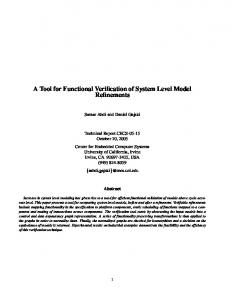
Figure 2. Visualization of various objects in MA Figure 2 shows how we visualize the various objects of MA. A behavior is represented by a rounded rectangle, while a channel is represented by an ellipse. Variables inside behaviors are represented by rectangular boxes. Note that hierarchical behaviors like bhier are shown by white rounded rectangles. Leaf level behaviors like blea f , that cannot be decomposed any further, are represented using colored rounded boxes. Identity behaviors like e are also shown as white rounded boxes. Ports are represented by
b < p >7→ I < p0 > where b < p > is the out-port of the writing behavior. The port I < p0 > on the parent behavior of b will eventually be bound to another blocking write relation or a channel transaction relation. 4
little rectangles on the circumference of the box for corresponding behavior. A port labeled p may be seen for behavior bhier in Figure 2.
p1
b1
v
b2
p2
(a)
b1 b1
b2
b2
q1
p1
q
q2 b
b1
a
c
a
p2
b2
(b)
b
Figure 4. Visualization of data flow via ports
(a)
(b) The channel transaction relation is illustrated in Figure 4(b). For now, let us consider only the simplest case of a channel transaction, that is a point-to-point transaction. Here, the port p1 of b1 uses the link a of channel c to write data. On the other side, port p2 of b2 uses the same link to read the data. The communication follows a double handshake protocol. The protocol guarantees that the receiver will wait until the sender is ready to write data. The sender on the other hand, will write data only upon the ready notification from the receiver. Hence, the channel semantics ensure that both the sender and receiver are synchronized at the time of the transaction.
Figure 3. Visualization of control flow relations in MA
4.4.1 Control flow Control flow relations are represented using broken directed edges as shown in Figure 3. A FSM-like control flow can be realized as shown in Figure 3(a). In this case, behavior b can start executing if either of the following conditions hold true: 1. b1 has completed and q1 evaluates to TRUE, OR 2. b2 has completed and q2 evaluates to TRUE.
p1
Such a control flow can be expressed in MA as a grouping of the two control terms as follows
a
p
b
a
c
a a
q1 : b1 ; b.q2 : b2 ; b
pn
A more complex control flow is realized by the generic control relation that involves synchronization. This case is illustrated in Figure 3(b). The AND-gate symbol is used to indicate the synchronization before behavior b can start executing. In other words, b may start executing only if both b1 and b2 have completed and q evaluates to TRUE. This instance of control flow can be expressed with a single term as follows q : b1 &b2 ; b
b1 bn
Figure 5. Visualization of multi-cast channel transaction
The more complex case of multi-cast channel transaction is shown in figure 5. The transaction consists of simultaneously sending the same data from a single sender to several receivers. For this reason, all the receiving behaviors and the sender must be executing concurrently. Also, a single address is used for a multi-cast transaction. The transaction link is visualized using a channel and the AND-gate symbol as shown in figure 5. The multi-cast communication still follows rendezvous semantics like the point-to-point communication. The difference is that instead of synchronizing two behaviors, all n + 1 participating behaviors must be synchronized. The transaction link as shown in figure 5 can be expressed in MA as a single term
4.4.2 Data flow Non-blocking communication takes place between behaviors using composition rules Rnw and Rnr . Essentially, behaviors read or write data to variables through their ports. The type of the port used and the variable should be the same for the relation to be valid. Figure 4(a) illustrates the non-blocking data flow from b1 to b2 via variable v. Behavior b1 uses its out-port p1 to write data to v, while b2 uses its in-port p2 to read data from v.
c < a >: b < p >7→ b1 < p1 > &b2 < p2 > ...&bn < pn > 5
5 Model Construction with MA
b par
b fsm vsp b
So far, we have seen the various objects and composition rules of MA. In this section, we look at how to construct hierarchical system models in MA. The objective is to represent models written in typical SLDLs using the objects and composition rules of MA. For simplicity, we will be using visual illustrations introduced in Section 4.4.
b1
(a)
Virtual Starting Point
b
vspb
fsm
b1
b2
q1 q'1
vtp b
vsp b
par
par
q2 b2 q'2
vtp b
fsm
(b)
Figure 7. (a)Parallel and (b)FSM style compositions of behaviors
q1
b1 b2
5.2 Parallel and Conditional Execution q2
Most SLDLs provide for special language constructs to create different types of behavioral hierarchies. The common ones are parallel composition and fsm-style composition. A sequential composition is simply a degenerate form of the fsm-composition. In MA, we can realize both these types of composition by using hierarchy and control relations. Figure 7(a) shows a parallel composition of behaviors b1 and b2 . A typical SLDL may allow construction of a parallel composition using a statement like par {run b1 ; run b2 }. Let the resulting behavior be called b par . The execution of b par indicates that both b1 and b2 are ready to execute. The execution of b par completes when both b1 and b2 have completed. In the corresponding MA expression, vspb par and vt pb par serve as the starting and terminating points, respectively, of the hierarchical behavior b par . We can see, that inside b par , b1 and b2 are allowed to start simultaneously. This is ensured by the control relations vspb par ; b1 .vspb par ; b2 Hence, the parallelism is realized by orthogonality of the execution of behaviors b1 and b2 . The control relation at the end b1 &b2 ; vt pb par ensures that both b1 and b2 must complete their execution before vt pb par executes. The execution of vt pb par indicates the completion of the hierarchical behavior b par . A typical FSM style composition of behaviors is shown in Figure 7(b). The control flow between behaviors is typically expressed using switch-case or goto constructs in SLDLs. A simple pseudo code example for a hierarchical behavior b f sm is as follows l1: run b1 ; if q1 == 1 goto l2 else break; l2: run b2 ; if q2 == 1 goto l1 else break; The control relations of b f sm can be written as follows in
vtp b Virtual Terminating Point
Figure 6. Control flow within hierarchical behaviors
5.1 Hierarchy Using the control flow relations, we can compose behaviors such that they execute in a desirable order. Most SLDLs provide for hierarchical compositions of behaviors to aid modeling. In MA, hierarchy is achieved using the interface object and its relation to behaviors. Figure 6 shows a hierarchical behavior b consisting of sub-behaviors b1 and b2 . The interface of b is visualized as the circumference of the box representing b. Note the virtual starting point(VSP) and the virtual terminating point(VTP) behaviors of b. The VSP is the identity behavior vspb that is the first to execute inside b. Other sub-behaviors of b are executed after vspb , depending on outgoing control relations from vspb . We can see in figure 6 that the VSP in this case vspb is triggering the execution of sub-behavior b1 . Due to its nature, a VSP behavior would only have outgoing control edges to other subbehaviors of b. Similarly, the identity behavior vt pb is the last behavior to execute inside b. In other words, the completion of b is indicated by the execution of vt pb . Due to its nature, the VTP behavior will only have incoming edges from other sub-behaviors of b. All hierarchical behaviors are assumed to have a unique VSP and a VTP. Hence, the starting and terminating control relations of b can be written as vspb ; b1 .b2 ; vt pb
6
the actual order of execution of concurrent behaviors and hence, it is not possible to tell if the receiving behavior will execute after the sender. To allow safe and predictable data transfer between behaviors, we use a channel transaction.
MA vspb par ; b1 .q1 : b1 ; b2 .q01 : b1 ; vt pb par . q2 : b2 ; b1 .q02 : b2 ; vt pb par
b hier
v1 b
out
b1
p2
p1
p1
b1
in
a
b'1
b2
a
c
p1'
p2'
a
b'2
a
b2
p2
v2
Figure 9. Blocking data flow bound to channel As in the case of non-blocking reads and write, MA provides mechanism for blocking reads and writes via ports. For instance, in Figure 9, we see a channel transaction from b1 to b2 over c. After zooming into the hierarchy of b1 and b2 , we see that the transaction is taking place from b01 to b02 . The port p1 of b1 makes the channel c visible to b01 . Therefore, using the relation
Figure 8. Using ports for non-blocking data flow in hierarchical behaviors
5.3 Variable Access via Ports In MA, as in most SLDLs, a variable is directly visible only to the behaviors that are at the same level of hierarchy as the variable itself. Therefore, in order to access variables at higher levels of hierarchy, data ports are used. As shown in Figure 8, behavior b1 reads variable v1 present in bhier via the port “in” of its parent b. Hence, to realized this port connection, we need terms at different levels of behavior hierarchy. At the level of bhier , we use the non-blocking relation v1 → b < in >
< a >: b01 < p01 >7→ I < p1 > behavior b01 can access channel c. However, this requires p1 to be bound to the virtual link addressed by a. Similarly, on the other side, sub-behavior b02 inside b2 , uses the blocking relation < a >: I < p2 >7→ b02 < p02 > to access the read method of c via port p2 . In this case, port p2 makes the channel c visible to b02 . As before, p2 must be bound to the virtual link addressed by a.
At the level of b, we use the port connection from the interface of b to b1 . We can write this as the relation
b
I < in >→ b1 < p1 > The dual of read port connection is the write port connection as shown by the access of variable v2 from behavior b2 in figure 8. In this case, the port “out” of b is used to realize the variable access. The term at the level of bhier is
p11
b1
a1
p11'
p1
a1
a1
b'1
c b2
a2
a2 p2
p22
a2 p22'
b'2
b < out >→ v2 while the term at the level of b is
Figure 10. Sharing channel for transactions with different addresses
b2 < p2 >→ I < out >
5.4 Channel Access via Ports
In MA several virtual links may share a single channel. Each of the virtual links are assigned a different address, but the data transfer takes place on the same medium. Figure 10 shows an instance of channel sharing. In this model, we have two virtual links with addresses < a1 > and < a2 >. Transactions may be attempted concurrently on these links. However, due to sharing of the channel, we can allow only one transaction at a time. This is a classic case of bus arbitration, where an arbiter ensures that only one transaction
Non-blocking communication is typically used for sequentially executing behaviors. The sender behavior writes to the communicating variable. The receiver behavior executes after the writer has completed and reads from the communicating variable. However, when behaviors are executing concurrently, such a method of communication would not be safe anymore. In other words, we cannot guarantee 7
The typical SLDL implementation of e1 would look like
v e1
in
b e h a v i o r e1 ( i n , o u t ) { i n t temp ; temp = i n ; o u t = temp ; };
out
v' (a)
v e2
in
p
out
c
a
a
b
The second case of identity behavior is shown in figure 11(b). Here, the “in” port is connected to a variable, hence the input is read using a non-blocking relation. On the other hand, the “out” port is connected to channel c. Hence, the output needs to be sent to b using a blocking write relation. In MA, the read/write relations of e2 are expressed as
(b)
b
p a
a
c
in
e3
out
v
v → e2 < in > .c < a >: e1 < out >7→ b < p >
(c)
b
p a
c
a in
e4
out
The typical SLDL implementation of e2 would be as follows a'
b e h a v i o r e2 ( i n , o u t ) { i n t temp ; temp = i n ; o u t . w r i t e ( a , temp ) ; };
p'
c'
b' a'
(d)
Figure 11. Various manifestations of the identity behavior
The third case of identity behavior is shown in figure 11(c). Here, the “in” port is connected to a channel c, hence the input is read from behavior b using a channel transaction. On the other hand, the “out” port is connected to variable v. Hence, the output needs to be written using a nonblocking write relation.In MA, the read/write relations of e3 are expressed as
may take place over a bus at any time. In MA, the same concept is implemented using mutual exclusion in the channel. The read and write methods of the channel implement a mutual exclusion policy, where the channel is a shared resource and each transaction is treated as a critical section. This allows us to connect several different virtual links to the same channel.
c < a >: b < p >7→ e3 < in > .e3 < out >→ v The typical SLDL implementation of e3 would be as follows b e h a v i o r e3 ( i n , o u t ) { i n t temp ; i n . r e a d ( a , & temp ) ; o u t = temp ; };
5.5 Using Identity Behaviors A class of behaviors in MA is known as the identity behavior. As the name suggests, these behaviors have the same output as the input. As a result they do not have any computation inside them. They have two ports namely the “in” port for reading the input and an “out” port for writing the output. In general, the identity behavior first reads data from the “in” port to a local variable and then writes this variable to the “out” port. The actual implementation of the read and write within the identity behavior depends on the port connections. There are four basic manifestations of the identity behavior as shown in figure 11. Let us assume that the data read and written by the identity behavior is of integer type. In the first case, as shown in figure 11(a), both the “in” and “out” ports of the identity behavior e1 are connected to variables. Hence, the respective read and write are non-blocking relations. In MA, the read/write relations of e1 are expressed as v → e1 < in > .e1 < out >→ v0
Finally, the fourth manifestation of identity behavior is shown in figure 11(d). Here, the “in” port of e4 is connected to a channel c for reading data from b. Hence the input is read using a channel transaction relation. The “out” port of e4 is also connected to a channel named c0 for writing data to b0 . Hence, the output is also written using a channel transaction relation. In MA, the read/write relations of e4 are expressed as c < a >: b < p >7→ e4 < in > .c0 < a0 >: e4 < out >7→ b0 < p0 > The typical SLDL implementation of e4 would be as follows b e h a v i o r e4 ( i n , o u t ) { i n t temp ; i n . r e a d ( a , & temp ) ; o u t . w r i t e ( a ’ , temp ) ; };
8
6 Hierarchical Modeling in MA
We can also see control flow relations that determine the execution scenario under the conditions labeled on the control arcs. We also see data flow relations, both amongst sub-behaviors and between sub-behaviors and the interface. The grouping of relations between local objects will be referred to as the internal terms of a hierarchical behavior. Similarly, the grouping of relations involving the interface will be referred to as the interface terms of the hierarchical behavior. We can write the hierarchical behavior as a grouping of all its internal and interface terms, along with the internal terms of its sub-behaviors. The grouping of internal terms for a given behavior b is represented as [b]. Thus, we can write [bhier ] = [vspbhier ].[b1 ].[b2 ].[vt pbhier ].vspbhier ; b1 . q1 : b1 ; b2 .q01 : b1 ; vt pbhier .b2 ; vt pbhier .b1 < p12 >→ v. v → b2 < p21 > The interface terms of bhier is represented by |bhier |. From figure 12, we can see that |bhier | =< a >: I < p1 >7→ b1 < p11 > . b2 < p22 >→ I < p2 > Finally, we write the hierarchical behavior as a grouping of its internal and interface terms. We will use the convention of enclosing the expression for a hierarchical behavior in braces. Therefore, we get bhier = ([bhier ].|bhier |)
The model of a system is a behavior in MA. Typically, it is a hierarchical behavior showing the various components and connections of the system and the functionality within these components. While modeling, it is imperative to provide the right amount of detail for analysis purposes. The granularity of the leaf level behaviors is an important factor in deciding if the model can be analyzed. Typically, leaf behaviors are treated as atomic by the model analysis and transformation tools. In one extreme case, a system model can be represented as a single leaf behavior. Although the model may simulate correctly, it is useless for performing any transformations. On the other hand, too much granularity may make design decisions too cumbersome. For example, each statement in the SLDL description may be treated as a leaf behavior. Such a description will present too many design choices, with only few of them being useful. Usually, the designer knows what functionality should not be distributed on different PEs. For instance, operations that work on the same set of data or use the same type of resources are grouped into one behavior.
6.1 Internal and Interface Terms As mentioned earlier, hierarchy is a key feature in SLDLs. Hierarchy allows us to compose systems in a modular way. In MA, it is possible to represent a behavior as a grouping of terms involving its sub-behaviors, its interface and its local variables and channels.
bhier
b par
vspb
b vsp b
p2
hier
a
hier
p1
par
c
a
b3
p31
1
b1
p11 a p12
q1
p1
v p
q1' p22
vtp b
par
p21
b2
Figure 13. Hierarchical behavior b par with a parallel composition
1
vtp b p2
hier
Figure 12. A hierarchical behavior with local objects and relations
6.2 Multiple Levels of Hierarchy In the above example, a fsm-like hierarchical composition was created. The resulting behavior bhier can be used further to create more hierarchical behaviors. For instance, in figure 13, we see behavior bhier in a parallel composition with behavior b3 . The two behaviors exchange data using
Figure 12 shows a hierarchical behavior bhier . The expression for the hierarchical behavior is written using the local objects and composition rule. For instance, in the given behavior bhier , we can see sub-behaviors b1 and b2 . 9
predecessor, it may be replaced by vt pbhier . This is because vt pbhier is always the last behavior to execute inside bhier . This allows us to define the first two laws for flattening a given hierarchical behavior b. The term on the LHS is part of the original expression involving b. The term of the RHS is the one that replaces the LHS term once b is flattened. We will use symbols x, yandz as free variables.
the virtual link addressed a, over channel c. The hierarchical composition results in a new behavior called b par . The expression for b par is written in MA as follows b par = ([vspb par ].[bhier ].b3 .[vt pb par ].vspb par ; bhier . vspb par ; b3 .bhier &b3 ; vt pb par . c < a >: b3 < p31 >7→ bhier < p1 > . bhier < p2 >→ I < p >)
FL 1 q : x ; b =⇒ q : x ; vspb
6.3 Flattening of Hierarchical Behaviors
FL 2 q : b ; x =⇒ q : vt pb ; x Hierarchy is only a modeling artifact in MA. Addition of hierarchy allows the designer to group different behaviors together. It does not add any functionality to the model. Unlike SLDLs, MA does not have different types of hierarchical compositions. Hierarchy by itself does not influence how a particular set of behaviors would execute. That execution order is already captured using the control flow and data transaction relations in MA. The usefulness of hierarchy comes in representing the structural entities in the model. For instance, in an architecture model, different PEs execute different sets of behaviors. These sets of behaviors are grouped into different hierarchical PE behaviors. vsp b
b par
vsp
b
To enable data flow, hierarchical behaviors allow for ports on their interface. These ports are essentially a conduit for data transfer from one leaf behavior to another. During flattening, these ports can be optimized away by appropriately making new port connections as shown in figure 14. A virtual link addressed a over channel c is used for blocking data transfer from b3 to b1 . However, due to the hierarchical behavior bhier , channel c is not visible from the local scope of b1 . Thus, the port p1 is used to facilitate the connection of b1 with channel c. When the interface of bhier disappears during flattening, we can directly connect channel c to b1 . Similarly, the port p2 on bhier can be optimized away by directly connecting b2 < p22 > to port p on b par interface. Therefore, we have the following additional laws for port optimization during behavior flattening. On the LHS, we show the expression for the hierarchical behavior enclosed in braces. Only the interface term for the relevant port is shown.
par
hier
p11
a
b1
c
p12
a
FL 3 (...y → I < p > ...) < p >→ x =⇒ y → x
b3 q1 q1'
p22
FL 4 x → (...I < p >→ y...) < p >=⇒ x → y >
p21
FL 5 z < a >: x 7→ (... < a >: I < p >7→ y...) < p >=⇒ z < a >: x 7→ y >
b2
vtp
p
p31
v
b
FL 6 z < a >: (... < a >: y 7→ I < p > ...) < p >7→ x =⇒ z < a >: y 7→ x >
hier
vtp b
6.4 Granularity of Leaf Behaviors par
From the verification perspective, it is important that the model should have a fine enough granularity of leaf behaviors. Recall that during analysis of system models, we treat leaf behaviors as atomic units. Channel transactions, and consequently blocking reads and writes, impose implicit control relations between communicating behaviors. Therefore, such communication points must be explicitly represented in the model description. Our goal is to clearly distinguish the control relation between two leaf behaviors. This relationship will form the basis for comparing two models for functional equivalence. If there is a leaf level behavior with a blocking read or write
Figure 14. Behavior b par after flattening of bhier For functional validation, we need to be concerned with only the leaf level behaviors. Hence, we may get rid of hierarchy by flattening the model. The laws for flattening a hierarchical behavior follow from the semantics of hierarchical behaviors in MA. Consider the hierarchical behavior bhier in figure 12. Now, by the semantics of the VSP, any control relation leading to bhier is effectively leading to vspbhier . This is because vspbhier is always the first behavior to execute inside bhier . Similarly, in any control relation where bhier is a 10
b
a
b1
flow inside b1 makes e1 execute before b12 . Therefore. in the above two scenarios, the execution order of leaf behaviors are different. Note that if both behaviors b1 and b2 were treated as leaf behaviors, the two scenarios shown in figure 16 could not be distinguished. Based on the above discussion, we can establish the simple rule for granularity of analyzable behaviors. We impose the modeling restriction that channel transaction relations or blocking data flow relations can involve only hierarchical behaviors or identity behaviors. Hence, after flattening the model may have channel transaction relations only between identity behaviors. In other words, in a completely flattened analyzable model, if there is a term c < a >: x 7→ y, then x, y ∈ B ε .
vspb
p1
a c p2
b2
vtp b
Figure 15. Leaf level behaviors communicating using channel c
7 Channel Semantics to a channel, then during execution it must wait at some unknown point to complete that blocking transaction. The lack of granularity, therefore, restricts us from knowing the actual order of computations. This problem is illustrated by a simple example in Figure 15. Consider a hierarchical behavior b formed by the parallel composition of leaf behaviors b1 and b2 . Behaviors b1 and b2 communicate in a rendezvous fashion, using channel c. Since leaf behaviors are atomic for our analysis, we cannot tell exactly when does the transaction over c take place. In other words, we cannot tell what part of b1 or b2 executes before the transaction and what part executes after it. By the execution semantics of the channel transaction, there is a control dependence between parts of b1 and b2 . However, due to the lack of granularity in the description, we cannot determine this dependence. The importance of granularity is further illustrated in Figure 16. This time we assume that behaviors b1 and b2 , from Figure 15, are hierarchical. Thus, the MA description now provides more details, so that the control ordering imposed by the transaction relation can be analyzed. Both b1 and b2 are sequentially composed. The channel is linked to identity behaviors on either side, namely e1 and e2 . By virtue of being identity behaviors, both e1 and e2 do not carry any computation. Therefore, for a channel transaction involving e1 and e2 , we need not be concerned about any hidden ordering of computation. Essentially, by the rendezvous semantics of the transaction, all execution preceding e1 also precedes all execution following e2 , and vice versa. In the first scenario, shown in Figure 16(a), we see that b12 inside behavior b1 executes before e1 . Considering the rendezvous semantics of the channel transaction, we can tell that b12 has no ordering with b21 . However, in the scenario shown in figure 16(b), the same rendezvous semantics force b21 to execute before b12 . This is because now, the control
The channel object allows for reliable communication between two concurrently executing behaviors. In an SLDL implementation, the channel uses events and data variable to implement a rendezvous communication protocol. As discussed before, a channel transaction implies a control dependency between parts of the communicating behaviors. Hence, we will assume both the sender and the receiver to be identity behaviors in future discussions. a
e wr
a c
out
in
e rd
time Case A: Writer arrives first
wait
Case B: Reader arrives first
wait
wr wait rd wr wait rd
Atomic Transaction
Figure 17. Timing diagram of a transaction on a channel
7.1 Channel with Single Virtual Link Figures 17 shows a transaction taking place over channel c. We can express this transaction MA using the term c < a >: ewr < out >7→ erd < in > 11
b
b
vsp b vsp b1
b2
b1
vsp b2
vsp b
b11
b2
b1
vsp b1
vsp b2
b11 b21
a b12 e1
a
p1
b21
a
a a
c
a
e1 out
p2 in
a
c
p1
p2
e2
vtp b2
e2
in
b12
out
vtp b1
a
vtp b1
vtp b2
vtp b
vtp b
(a)
(b)
Figure 16. Different scenarios for transaction over c (a) b12 executing before e1 , and (b) b12 executing after e1 The timing diagram for this channel transaction shows two instances of execution. In the first instance, called Case A, the writer reaches the communication point before the reader. By this we mean that during model execution, ewr is scheduled to execute before erd . However, the rendezvous semantics dictate that ewr must wait until erd is ready before executing. It may be noted that if there is a control dependency from ewr to erd , the resulting model would deadlock. Hence, erd must be allowed to start independently of ewr and vice versa. Once erd is ready to start the transaction, it notifies ewr . The transaction is thus initiated by ewr , that performs a write on the local memory of the channel. Subsequently, erd reads the data from this memory. In the second execution scenario, called Case B, the reader is scheduled before the writer is ready. This forces erd to wait until ewr is ready to start executing. The shaded part of the execution, in the timing diagram, indicates the atomic nature of the transaction. Note that the channel resources (i.e. its local memory) are occupied only during the actual reading and writing of the data.
e1
in
out
a1
a1
e1'
c
e2
a2
a2
out
in
e2'
time Arrival times
e1
e1' e2 e2'
Wait1 Transaction times
Wait2 wr(a1) rd(a1)
wait wr(a2) rd(a2)
Atomic Transaction
Figure 18. Multiple simultaneous transactions on a single channel
7.2 Channels with Multiple Virtual Links is to allow greater bandwidth on the channel. Consider the configuration shown in figure 18. In this case, two virtual links, addressed a1 and a2 , are shared over channel c. These links can be written as a grouping of the following terms c < a1 >: e1 < out >7→ e01 < in > . c < a2 >: e2 < out >7→ e02 < in > The timing diagram shows the actual arrival schedule of the four communicating identity behaviors and the resulting communication schedule on the channel. Note that de-
As discussed earlier, channel sharing is possible for different virtual links, but the transactions are scheduled sequentially. This mutual exclusivity of transactions can be achieved by the use of semaphore (or test and set) constructs in SLDL. Thus, the shaded part representing the actual data read and write over the local memory of channel is mutually exclusive. The reason why we do not make the entire transaction (including synchronization) mutually exclusive 12
2. Any behavior following the receiver identity behavior would not execute until the sender identity behavior has executed.
spite the fact that e1 arrives first, transaction on a2 takes place before that on a1 . This is because, the data transfer of transaction on a2 is ready to be performed before that for a1 . Thus, the data transfers on the channel are scheduled on first-ready first-serve basis. Although the transaction on a1 is ready to be performed when e01 arrives, it must wait for the duration wait2 since the transaction on a2 is in progress. a
e1
e1
a
If we were to optimize away the channel to extract only the control dependencies, the result will be as shown in figure 19. As per the above premises, behavior b1 following sender e1 cannot start until e2 has completed. This is guaranteed by including the term
e2
e2
c
q1
q1 : e1 &e2 ; b1
q2
b1
q1
q2
In the dual of the above case, b2 following e2 is blocked until the sender e1 has executed. This premise is ensured by the term q2 : e2 &e1 ; b2
b2 b1
b2
(a) a
e1
a c
e1
e2
q1
q2
b1
q2
q1
b2
Figure 19(b) shows the general case, where the behaviors following the sender and the receiver may already have several predecessors. In that case, the new predecessor (e1 for b2 and e2 for b1 ) is simply added to the list of predecessors in the corresponding blocking relation.
e2
b1
b2
8 Execution Semantics
(b)
In order to define the execution semantics of MA, we first introduce the underlying model of computation. The control flow in the model is captured using the Behavior control graph(BCG). BCG is similar to the popular computation model of Kahn process network (KPN). KPN is a directed graph, where nodes represent processes and edges represent unbounded FIFO queues. Each edge is directed from the writer to the reader process. Also, writes are unblocked, while reads are blocking. This means that the reading process must wait until the queue the required amount of data for the reader process to execute. Note that all queues have only one reader and only one writer, and that the queues are the medium for data transfer between processes. KPN can effectively model concurrency and synchronization, but they are not useful for modeling non-determinate behavior or conditional control flow. The data flow in the model is captured using the Port Connection Network (PCN), which is a net-list of behaviors, variables and control conditions, with directed arcs denoting the data dependencies amongst them. Together, the BCG and the PCN are used to define the execution semantics of the model.
Figure 19. Resolution of channels into control dependencies
7.3 Control Flow Resolution of Links As seen during the discussion of channel semantics, the channels in MA imply control flow dependencies between communicating behaviors. Our eventual goal is collect all control dependencies between behaviors to form a monolithic control flow graph of behaviors. We will now see how to resolve the virtual links in flattened MA models into control dependencies. Figure 19 demonstrates this control dependency extraction. Recall that in an analyzable model, blocking relations and channel transaction relations can involve only identity behaviors or hierarchical behaviors. Upon flattening, the analyzable model would only have channel transaction relations between identity behaviors. Thus, for the purpose of control flow extraction from channel transaction relations, we need to consider only the case where sender and receiver are both identity behaviors. The synchronization properties of a channel would ensure the following two premises:
8.1 Behavior Control Graph The BCG is similar in principle to the Kahn Process Network [10], but with some remarkable differences.It is a directed graph (N,E) with two types of nodes, namely behavior nodes(NB ) and control nodes(NQ ). The behavior nodes, as the name suggests, indicate behavior execution, while the
1. Any behavior following the sender identity behavior would not execute until the receiver identity behavior has executed. 13
q1
b1_queue
b1
b1
_q
q 1 '_
b1
tion 6.3. We also saw the control relations that may result from a communication channel. After, flattening the model and extracting the control dependencies, we are left with a set of leaf level behaviors and control relations amongst them. This can be directly translated into a BCG in a trivial fashion. For each leaf behavior, we introduce a behavior node in the BCG, labeled by the leaf behavior’s id. For each control relation, we introduce a control node in the BCG, labeled by the control condition id. Also, edges are added to the BCG depending on the control relation. For instance, a control relation of the form
ue ue q1'
_q n'_ qu
eu
qm
e qn'
bk bk_q
n _q u
eue
q : b1 ; b2
Figure 20. The firing semantics of BCG nodes
would imply two directed edges (b1 , q) and (q, b2 ) in the BCG. On the other hand, a control relation of the form
control nodes evaluate control conditions that lead to further behavior executions. Directed edges are allowed from behavior nodes to control nodes and vice versa. Also, a control node can have one, and only one, out going edge. Thus, E(BCG) ⊂ NB (BCG) × NQ (BCG) ∪ NQ (BCG) × NB(BCG) The execution of a behavior node, and similarly, evaluation in a control node, will be referred to as a firing. Node firings are facilitated by tokens that circulate in the queues of the BCG as shown in Figure 20. Each behavior node (shown by rounded edged box) in the BCG has one queue, for instance b1 queue for behavior node b1 . All incoming edges to a behavior node represent the various writers to the queue. A behavior node blocks on an empty queue and fires if there is at least one token in its queue. Upon firing, one token is dequeued from the node’s queue. The control node (shown by circular node), on the other hand, has as many queues as the number of incoming edges. For instance qn has k queues, one each for edges from b1 through bk . A control node, sequentially checks all its queues and blocks on empty queues. If the queue is not empty, it dequeues a token from the queue and proceeds to check the next queue. The node fires after it has dequeued one token from each of its queues. After firing, a behavior node generates as many tokens as its out-degree, and each token is written to the corresponding queue of the destination control node in a non-blocking fashion. Upon firing, the control node evaluates its condition. If the condition evaluates to TRUE, then a token is generated and written to the queue of the destination behavior node.
q : b1 &b2 ...&bn ; b would imply n + 1 directed edges (b1 , q), (b2 , q),...,(bn , q) and (q, b) in the resulting BCG. Recall that each hierarchical behavior has unique vsp and vtp identity behaviors. Let us assume that the top level behavior in the model is called m. Then vspm is the first node to fire in the BCG of m. Therefore, m may be simulated by placing a single token in the queue for vspm . The simulation terminates when there are no more tokens left to be consumed. In other words, if all the FIFOs in the BCG are empty, then the execution has terminated. b p
v
v'
p11
q
p12
b1
p21
b2
Figure 21. Port connection network showing data dependencies
8.3 Port Connection Network The PCN is a directed graph which has three types of nodes, namely behavior nodes (NB ), condition nodes (NQ ) and variable nodes (NV ). The edges represent data dependencies in the model and are labeled using the port names involved in the dependency as shown in Figure 21. For instance, a directed edge from a behavior node b to a variable node v (shown by rectangular box), labeled p (written (b, v, p)) would mean that b writes to the storage indicated by v via its out-port p. Similarly, an edge from a variable node v0 to a behavior node b0 , labeled p0 (written (v0 , b0 , p0 ))
8.2 Deriving BCG from MA Expression Now that we have described the BCG, we can create a unique BCG from a given MA expression. This will allow us to establish the execution semantics of MA. We have seen how to create a flattened behavior for a model in sec14
would indicate that b0 reads variable v0 using its in port p0 . Note that for each variable v, there can be only one writer behavior (written as wr(v)). Control conditions also create data dependencies in the model. Thus, if a control condition q is a boolean function call q = fb (v1 , v2 , ..., vn ), then the node representing q has a directed edge from all the n variable nodes v1 thorough vn .
case, we need a notion of functional equivalence of models in MA. Using these notions, we can build tools for checking if two MA models are functionally equivalent. In this section, we will define our notion of equivalence and the algorithms needed for comparison of models based on such notion.
9.1 Notion of Functional Equivalence 8.4 Deriving PCN from MA Expression Our notion of functional equivalence is based on the trace of values that the variables hold during model execution. In particular, we are interested in the variables that are written to by non-identity behaviors. We will refer to such variables as observed variables. The reasoning is that variables that are connected to the output ports of identity behaviors are simply a copy of another variable. Informally speaking, we consider two models to be functionally equivalent, if they have identical observed variables and the trace of values assumed by those variables during model execution is identical, given the same initial assignment. The formal notion of equivalence is as follows. Given a model M, let I(M) be the initial assignment of observed variables in M. Let ∀v ∈ NV (PCN(M)), ∃wr(v) ∈ NB (PCN(M)) Let di , i > 0 be the value written to v after the ith execution of wr(v). Let d0 be the initial assignment value of v. We define the ordered set τ(v, M, I(M)) = {d0, d1 , d2 , ...} We claim that two models M and M 0 are equivalent iff ∀v, I(M) = I(M 0 ) ⇒ τ(v, M, I(M)) = τ(v, M 0 , I(M 0 )) From the above discussion, we have the following implications on equivalence checking using BCG and PCN. For two models, say M and M’, to be functionally equivalent, they must have
In MA, a non-blocking write is represented by the relation b < p >→ v In a PCN, this results in a directed edge from a behavior node b to a variable node v would mean that b writes to the storage indicated by v. The edge label p indicates the out port used by b for writing v. Similarly, the non-blocking read relation v0 → b 0 < p 0 > results in an edge from a variable node v0 to a behavior node b0 , labeled p0 , indicating that b0 reads variable v0 using its in port p0 . We must note that for each variable, there can be only one writer behavior. The restriction of having a single writer behavior for each variable would simplify modeling and analysis, since we do not have to deal with hazards related with multiple writers. Finally, the channels are also impose edges in the PCN. In the flattened form, we would expect to see channel relations only between identity behaviors. A channel transaction, represented by the MA relation c < a >: e1 < out >7→ e2 < in > will result in a directed edge from e1 to e2 in the PCN. A multi-cast transaction of the type
1. A one to one mapping of leaf level behaviors,
c < a >: e < out >7→ e1 < in > &e2 < in > &...&en < in >
2. A one to one mapping of observed variables, and
will result in n edges in the PCN, each such edge originating at e and terminating at nodes e1 through en .
3. Identical firing order for any two behaviors with data dependence.
9 Equivalence Checking of Models
9.2 Graph Reduction
The motivation behind MA is to enable the functional verification of various model transformations taking place during system level design. As a result of every design decision, the system model is transformed to reflect the properties imposed by the design decision. However, we must be able to ensure that the original intended functionality has not changed as a result of this transformation. We can ensure this either by using only proven correct transformations, or by having an equivalence checking tool to verify the models before and after the transformation. In either
For building an automated tool for equivalence checking, we need to define methods for reducing two models to a normal form representation. The reduction procedure must preserve the functionality of the model, as per the above notion. If the normal form of two models is identical, we can claim that the models are functionally equivalent. Otherwise, the result is inconclusive. Let us now consider some functionality preserving transformations to a model that will lead to its normal form. We will perform these transformations on the BCG and PCN 15
variables q1 and q2 ). However, it must be noted that as a result of elimination of e, the variable that e was writing to, also becomes invalid. This variable v2 is shown in the PCN in figure 22(a). Now, variable v2 is simply a copy of v1 , by definition of the identity behavior. Therefore, all dependencies on v2 , including in-port connections for behaviors and parameters for control conditions, must be replaced by dependencies on v1 . The elimination of e from the original model results in the PCN shown in figure 22(b). This simple example of identity elimination shows how the reduction rule works in principle. We now present the general definition of the rule.
representations of the model. We choose these graph representations to demonstrate the transformations for sake of clarity. The transformations can also be shown on corresponding MA expressions, since the two representations have one-to-one mapping. Our goal is to eliminate identity behavior nodes and redundant dependencies from the BCG and PCN, as the model is reduced to its normal form. Redundant dependencies include control dependencies that do not influence the value trace of the observed variables. 9.2.1 Identity elimination The identity behavior, by definition, does not perform any computation. Hence, we may remove the identity behaviors from BCG and PCN, while making appropriate changes to the variable dependencies. b1
v3 p3
v4
Given a model M, let e ∈ NB (M) be an identity behavior. Let M’ be the model resulting from elimination of e. Let there be m edges to e from control nodes q1 through qm in BCG(M). Also, let there be n edges from e to control nodes labeled q01 through q0n in BCG. Now, ∀i, j, s.t.1 ≤ i ≤ m, 1 ≤ j≤n In BCG(M), qi has in-degree l(i) and q0j has in-degree k( j) + 1. Let, (xi1 , qi ), (xi2 , qi ), ..., (xil(i) , qi ) ∈ E(BCG(M)), and
v5
v1
q1
in
b3
Identity elimination rule (R1)
q1
q2
e
e
out v2
q2
p4
b2
(e, q0j ), (y1 , q0j ), ..., (yk( j) , q0j ) ∈ E(BCG) Also, let (q0j , z j ) ∈ E(BCG). After, elimination of e, the merger of control nodes would result in m × n new control nodes. Therefore, ∀i, j, s.t.1 ≤ i ≤ m, 1 ≤ j ≤ n j j qi ∧ q0j : xi1 &...&xil(i) &y1 &...&yk( j) ; z j ∈ BCG(M 0 ) In the PCN, if (e0 , e), (e, v, out) ∈ PCN(M), e0 ∈ B I , then PCN(M 0 ) = (PCN(M) − (e0 , e)) ∪ (e0 , v, out). If (v, e, in), (e, v0 , out) ∈ PCN(M), then ∀x, s.t.(v0 , x, p) ∈ PCN(M) PCN(M 0 ) = (PCN(M) − (v0 , x, p)) ∪ (v, x, p). j
b4
q3
BCG
PCN
(a) Before applying identity elimination
b1 v3
v4
v5
v1 q1
q2
p4
p3 q3
b2
BCG
b3
b4
q1
q2
j
PCN b1
(b) After applying identity elimination q dominator path
Figure 22. Parts of BCG and PCN before and after identity elimination
b
b2
(a) BCG before redundant control elimination
The simple example illustrated in figure 22(b) shows parts of the BCG and PCN involving an identity behavior e. In the BCG, e is part of the control path from b1 to b2 . It must be noted that there are no other edges to either e or the control nodes q1 and q2 . As per the semantics of BCG, we can eliminate e by merging the control nodes q1 and q2 as shown for the BCG in figure 22(b). Note that in both the models, b2 will execute after b1 if both control conditions q1 and q2 evaluate to TRUE. Hence, the elimination of e leads to the merging of nodes q1 and q2 to form the new control node labeled as q1 ∧q2 (ANDing of the boolean
b1 q dominator path
b
b2
(b) BCG after redundant control elimination
Figure 23. BCG before and after redundant control elimination
16
between b2 and q2 , then changing the order of firing between b2 and q2 , or b2 and b3 would not change the value trace for any variable in M. Therefore, the artificial control dependency from b2 to q2 may be removed, as illustrated in figure 24. However, the rule applies only if the nodes q1 and b2 must have an in-degree of 1, while the node b3 has an out-degree of 1. With these restrictions, dom(b2 , M) = b1 ∪ dom(b1 , M). Thus, firing of b1 will enqueue a token on the queue for b3 if q2 is TRUE. Also, the token released by firing of b2 must be enqueued to q3 if the edge (b2 , q2 ) is to be removed. Hence, the transformation illustrated in Figure 24 is functionally correct under the given restrictions.
9.2.2 Redundant control dependency elimination In order to eliminate spurious edges in a BCG, we first need a control dependence analysis. Given model M, let y ∈ NB (BCG(M)), x ∈ N(BCG(M)). If during any execution of M, y always fires at least once between every firing of x, then we define y to be a dominator of x. The set of dominator nodes for x will be represented by dom(x, M). The set dom(x, M) can be defined inductively as follows 1. If x ∈ NB (BCG), then dom(x, M) = dom(x, M) ∪ T (q,x)∈E(BCG(M)) {y : y ∈ dom(q, M)} 2. If x ∈ NQ (BCG), then dom(x, M) = dom(x, M) ∪ S (b,x)∈E(BCG(M)) {b ∪ {y : y ∈ dom(b, M)}}
Control relaxation rule (R3)
An instance of control dependency elimination is shown in Figure 23. Given q ∈ NQ (BCG(M)). Let b1 , b2 ∈ NB (BCG) and (b1 , q), (b2 , q) ∈ E(BCG) Thus b1 and b2 must fire for q to fire.If we can show that b1 ∈ dom(b2 , M) then the edge (b1 , q) can be eliminated from the BCG. This is because, upon execution of b1 , a token will be enqueued in the queue corresponding to (b1 , q). Now, if b2 executes, we know that b1 has already executed and enqueued the relevant token. The node q will dequeue this token from b1 and will wait for a token from b2 . Hence, a token from b2 means that b1 must already have a token sent to q. If we remove edge (b1 , q), while keeping edge (b2 , q), the order of firings in BCG would not change.
Given model M, let (b2 , q2 ), (q2 , b3 ), (b1 , q1 ), (q1 , b2 ), (b3 , q3 ) ∈ E(BCG(M)). If the following conditions hold 1. 6 ∃b 6= b1 , s.t. (b, q1 ) ∈ E(BCG(M)), and 2. 6 ∃q 6= q1 , s.t. (q, b2 ) ∈ E(BCG(M)) and 3. 6 ∃b0 6= b3 , s.t. (b0 , q3 ) ∈ E(BCG(M)) and 4. 6 ∃v, p, p0 ∈ N(PCN(M)), s.t. (b2 , v, p), (v, q2 ), (v, b3 , p0 ) ∈ E(PCN(M)) then E(BCG(M)) = E(BCG(M))∪{(b1 , q2 ), (b2 , q3 )}−(b2 , q2 ).
Redundant control dependency elimination rule (R2) Given model M, let q ∈ NQ (BCG(M)). If ∃b1 , b2 ∈ NB (BCG(M)), s.t. b1 ∈ dom(b2 , M) and (b1 , q), (b2 , q) ∈ E(BCG(M)), then E(BCG(M)) = E(BCG(M)) − (b1 , q). b1
q1
b2
q2
b3
q1
b2
b3
q2
(a) Original BCG without in/out degree restrictions
q3
(a) BCG before edge relaxation q1
b1
q1
b2
q2
b3
q3
e1
1
b2
q2
b3
e2
1
(b) BCG after addition of identity behaviors e1 and e2
(b) BCG after relaxation of edge (b2, q2) q1
Figure 24. Control relaxation for edge (b2 , q2 )
e1
1
b2
q2
b3
1
e2
(c) BCG after relaxation of edge (b2, q2)
9.2.3 Control relaxation
Figure 25. Control relaxation for edge (b2 , q2 ) without in and out-degree restrictions
Figure 24 illustrates the control relaxation rule. Given model M, let (b2 , q2 ) and (q2 , b3 ) be edges in the BCG of M. If there is no data dependency between b2 and b3 and 17
consists of rearrangement and/or replacement of objects in the input model to create an output model. Each of the design decisions result in different types of transformations. For different types of transformations, we need a different verification technique to validate it. We will follow the system level design methodology, as shown in Figure 1. The following design steps are encountered as we start from a functional specification model and produce a scheduled transaction level model.
Control relaxation can be further generalized by removing the restrictions on the in-degree of b2 and q1 and the out-degree of b3 . The original BCG, with arbitrary degrees for the relevant nodes can be transformed as shown in figure 25. Using the inverse of rule on identity elimination, we can add identity behaviors e1 and e2 before b2 and after b3 , respectively. This would allow us to use the control relaxation transformation to derive the BCG shown in the midle of figure 25. Finally, after control relaxation, the identity reduction rule can be applied to optimize away e1 and e2 .
1. Behavior partitioning
9.3 Comparison of MA Models
2. Static scheduling
In order to validate functional equivalence of M and M’, we convert their BCG and PCN to the normal form. The normal form of M is derived by iteratively applying the reduction rules to the BCG(M), PCN(M) pair until none of the rules is applicable anymore. The resulting normal form graphs are represented by NBCG(M) and NPCN(M). Similarly, we derive the normal form graphs for M’. If NBCG(M) is identical to NBCG(M’) and NPCN(M) is identical to NPCN(M’), then M is equivalent to M’. This follows from transitivity of the equivalence relation and the functionality preserving nature of the reduction rules. In the following sections, we will look at the verification requirements at each stage of system level design. We will also present the application of our equivalence checking method for some of these design steps using simple examples.
3. RTOS insertion 4. Bus insertion We will now look at the model transformations resulting from these design decisions and the requirements for verifying those transformations.
10.1 Behavior Partitioning A given specification consists of an arbitrary hierarchy of behaviors. During partitioning, we determine the number of PEs that will be needed to implement the design. The leaf behaviors in the specification are then distributed over these PEs. The PEs are assumed to execute concurrently. Thus, in this step, the design decision is to map each leaf behavior in the specification model to a PE. The output model must follow a well defined template to reflect the mapping decision. The output shows the PEs as a parallel composition of hierarchical behaviors. Each PE behavior is composed from the leaf level behaviors that were mapped to it. Hence, the transformation produces a rearrangement of behaviors. Additional channels are added from the library for synchronization amongst behaviors. We need this synchronization since the original order of execution of the leaf behaviors must be maintained in the new model as well. The data flow relations in the original model must also be modified to reflect the locality of memory in each PE. The original data transfers between leaf behaviors, mapped to different PEs, will now go across PEs. Hence, they must be routed via identity behaviors using channels. Figure 27 shows a simple specification model M on the LHS with two behaviors b1 and b2 and condition control flow. After the execution of b1 , if condition q evaluates to TRUE, then b2 is executed, else the execution terminates. On the RHS, we see an architecture level implementation M 0 where b1 is assigned to PE1 and b2 is assigned to PE2 . Identity behaviors n and w are added along with rendezvous channel sync to preserve the original control flow. Since the transformations consist of rearrangements and addition of identity behaviors and channels, equivalence
Library of Objects ( channels/ behaviors)
Input Model (SLDL)
Design Decisions (GUI)
Model Transformation
Equivalence Checker
Output Model (SLDL)
Figure 26. Automatic equivalence checking of system level models
10 System Level Verification Methodology Figure 26 shows the methodology for generating a refined SLDL model from the input and checking the functional equivalence of the two models. The model generation algorithm uses the design decisions and syntactically transforms the input model. The transformation essentially 18
q'
execute, execution inside PE1 will stall, as it waits for the data transaction. Behavior b2 may be scheduled before the transaction, if it has no data dependency on b3 . The resulting schedule,shown in 28(b), optimizes timing. Since, the static scheduling process changes only the control dependencies, the leaf level behaviors in input and output models should match. As in partitioning, we do not add any new non-identity leaf behaviors to the model. Therefore, equivalence checking is also applicable in this design step.
M’
M
PE1
PE2
b1
b1 q b2
w sync1
n q'
q b2
Figure 27. Model generation after behavior partitioning
10.3 RTOS Insertion checking would work for this transformation. Note that in this step, we do not add any new non-identity leaf behaviors to the model. Hence, the equivalence checker can resolve the new objects in the model.
As explained above, static scheduling is one way of serialization of behaviors in a model. However, PEs that implement software may provide for dynamic scheduling. In this case, the non-determinism of concurrency is resolved at execution time. In a parallel composition of behaviors, the ordering of behavior execution is done during run time. This ordering is performed by a scheduler that is part of the PE’s operating system. In a SLDL implementation, the scheduler is another behavior that models the Real Time Operating System (RTOS). The concurrent behaviors are then modified to make calls to the OS behavior, before starting execution. If a behavior is scheduled for execution, it is notified by the scheduler. Upon completion, the behavior must notify its completion to the RTOS and release the PE resources. Competing scheduler requests are resolved using a scheduling policy. Most of these policies are well known like EDF, Round Robin, FIFS etc. Essentially, during RTOS insertion, the dynamic scheduling policy of the SLDL simulator is replaced by that of the explicit RTOS. The addition of a new non-identity behavior (in this case, the scheduler) renders our equivalence checker unusable. Therefore, for dynamic scheduling, we need to ensure that the scheduler behavior, and hence the scheduling policy, satisfies the same properties as the scheduler of the SLDL simulator. This can be verified using a property verification tool. If the property verification is successful, the scheduler behavior can be abstracted away from the model. The MA expression during this SLDL transformation can, thus, remain unchanged if the dynamic scheduler of the RTOS follows the simulator’s properties.
10.2 Static Scheduling Static scheduling is performed in system level models either due to resource constraints or timing optimization. Behaviors mapped to HW are typically targeted for implementation with a single controller. As a result, any parallelism in the HW PEs must be serialized statically. Consider an unscheduled HW PE with two threads of execution. The first thread executes behavior b1 followed by b2 , while the second thread executes b3 followed by b4 . A possible serialization of the PE would sequentially execute the behaviors in the order {b1 , b3 , b2 , b4 }. Other schedules are also possible as long as they do not violate data dependencies. c PE1 ……... run (b1) c.send (d) run (b2) ………
c PE2 ……... run (b3) c.recv (&d) ………
(a)
PE1 ……... run (b1) run (b2) c.send (d) ………
PE2 ……... run (b3) c.recv (&d) ………
(b)
Figure 28. Different communication schedules for transaction over channel c.
10.4 Bus Insertion Reordering of behaviors can also take place as a result of communication scheduling. Such a scenario is shown in Figure 28, where data d is sent from PE1 to PE2 over channel c. The channel implements rendezvous communication semantics, i.e. both sender and receiver must synchronize for the transaction to take place. Consequently, for the case shown in Figure 28(a), b2 must wait until b3 has completed and the transaction is performed. If b3 takes a long time to
After behavior partitioning and scheduling, the system model consists of concurrent behaviors communicating with several channels. Although, the model shows the computation structure correctly, the communication structure still needs to be implemented. In a bus-based SoC communication scheme, the various PEs are connected to system busses. The communication model can thus be rep19
resented using channels for busses. All virtual links in the input model are shared over the new bus channels. The design decision in this case is choosing the number of bus channels and mapping the virtual links to the bus channels. Also, the ordering of transactions on the bus may be done using an arbitration policy. By default, in MA, we follow a first-come first-serve policy as explained in Section 7.2. However, if the designer chooses to use a different scheduling, he or she may add a new arbiter behavior to schedule transactions over a bus. The arbitration of transactions is analogous to dynamic scheduling of behaviors, described above. For verification, we have the same scenario as that in RTOS insertion. Equivalence checking is not directly applicable since the output model has a new non-identity leaf behavior. As before, we can use property checking to verify that the arbitration policy preserves the functionality of the model. If we can prove, using a property checking tool, that the arbiter behavior will
M
q'
vsp m p1
b1 q b2
v p2
vtp m
vspm
b1 p1
1
v p2
b1
q'
q q
vtp m
q'
b2
b2
1
PCN(M)
BCG(M)
Figure 29. Example of a simple specification model and its graph representations
1. never cause a deadlock 2. eventually schedule a transaction request
M’
then we can abstract it away.
vsp
PE1
m'
PE2
vsp pe1
p1
11 Case Study: Verification of Behavior Partitioning
b1
p1'
v in
vsp
in
n
a
c
a
a
w
p2'
q b2
a out
pe2
out
v' p2
q' vtp pe1
In this section, we will use a simple example to demonstrate functional equivalence checking of models before and after behavior partitioning. We start by capturing the specification and (partitioned) architecture model as hierarchical behaviors in MA. The models are flattened using the flattening laws described in Section 6.3. Then, we resolve the channels and derive the BCG and PCN for the two models. Finally, we use the reduction rules in Section 9.2 to obtain the normal form graphs for the models. The isomorphism of the normal form graphs is used to check the equivalence of the specification and architecture models.
vtp pe2
vtp
m'
Figure 30. Architecture model derived after partitioning
Let us assign two PEs, namely PE1 and PE2 to implement this specification. Also, let us map b1 to PE1 and b2 to PE2. A possible architecture model M 0 , created from the specification and the mapping decision, is shown in Figure 30. Note that additional hierarchy is created for PE1 and PE2, which execute in parallel. New identity behaviors n and w are introduced in PE1 and PE2, respectively. These identity behaviors are used to send data in variable v from PE1 to PE2, via the channel c. This data is needed by b2 and the control conditions q and q0 . Note that the data from v is copied into variable v0 , which is local to PE2. In MA, the architecture model can be written using the following expressions. M 0 = [vspm0 ].[vt pm0 ].[pe1 ].[pe2 ].vspm0 ; pe1 . vspm0 ; pe2 .pe1 &pe2 ; vt pm0 . c < a >: pe1 < p01 >7→ pe2 < p02 >
11.1 Specification and Architecture Models The specification model M, shown in figure 29 is composed of two leaf level behaviors b1 and b2 and variable v, which is written by b1 and read by b2 . The following pseudo code describes the specification M: begin;run b1 ; if v < 5 run b2 ;end Assume that b1 uses port p1 to write v and b2 uses port p2 to read v. Also, let q = v < 5 and q0 = v ≥ 5. The MA expression for M can be written as follows: M = [vspm ].[vt pm ].[b1 ].[b2 ].b1 < p1 >→ v.v → b2 < p2 > .vspm ; b1 .q : b1 ; b2 .q0 : b1 ; vt pm .b2 ; vt pm 20
that w now reads directly from v via its in port. Similarly, in step 3, node w is optimized away using R1. Hence, all edges from w are replaced by those from vspm0 in the BCG. In the PCN, this reduction results in node w and v0 being optimized away. All edges from v0 are now converted to edges from v. Step 4 uses redundant control elimination rule R2 to get rid of redundant edges from vspm0 in the BCG. It may be noted that by definition of dominator in Section 9.2.2, we have vspm0 ∈ dom(b1, M 0 ) Note that in the BCG after Step 3, nodes labeled q, q0 and 1 have control dependencies from both b1 and vspm0 . Since, vspm0 is a dominator of b1 , we can eliminate the edges (vspm0 , 1), (vspm0 , q) and (vspm0 , q0 ). There are no changes to the PCN. In Step 5, we use R1 once again to eliminate identity behaviors vt ppe1 and vt p pe2 from the BCG. Again, the PCN remains unchanged since these behaviors do not have any data dependencies. Finally, in step 6, we use R2 to get rid of edge (b1 , 1). This is possible because, from the definition of dominator, we can see that b1 ∈ dom(b2 , M 0 ). Again, the PCN remains unchanged. The BCG and PCN obtained after Step 6 cannot be reduced any further and, thus, represent the normal form for the architecture model M’. The normal form graphs of M’ are identical to the BCG and PCN of corresponding specification model M, shown in Figure 29(b). Hence, we have shown the function equivalence of the two models before and after mapping of specification behaviors to PEs for our example.
pe1 = [vsp pe1 ].[vt p pe1 ].[b1 ].[n].vsp pe1 ; b1 .b1 ; n. n ; vt p pe1 .b1 < p1 >→ v.v → n < in > . < a >: n < out >7→ I < p01 > pe2 = [vsp pe2 ].[vt p pe2 ].[w].[b2 ].vsp pe2 ; w. q : w ; b2 .q0 : w ; vt p pe2 .b2 ; vt p pe2 . < a >: I < p02 >7→ w.w < out >→ v0 .v0 → b2 < p2 >
11.2 Flattening of Models The specification model has only one level of hierarchy, so it cannot be flattened any further. The architecture model, on the other hand, has two levels of hierarchy. Therefore, we can flatten the architecture model to remove the hierarchy created by behaviors pe1 and pe2 . Using the laws in Section 6.3, the flattened architecture model can be expressed in MA as follows M 0 = [vspm0 ].[vt pm0 ].[vsp pe1 ].[vt p pe1 ].[b1 ].[n]. [vsp pe2 ].[vt p pe2 ].[w].[b2 ]. vspm0 ; vsp pe1 .vspm0 ; vsp pe2 .vt p pe1 &vt p pe2 ; vt pm0 . vsp pe1 ; b1 .b1 ; n.n ; vt p pe1 . vsp pe2 ; w.q : w ; b2 .q0 : w ; vt p pe2 . b2 ; vt p pe2 .b1 < p1 >→ v.v → n < in > . w < out >→ v0 .v0 → b2 < p2 > . c < a >: n < out >7→ w < in >
11.3 Reduction to Normal Form
12 Related Work
We will now use the reduction rules in Section 9.2 to derive the normal form representation of the two models. Let us start by considering the architecture model. Channel c in the flattened MA expression of M’ can be resolved into edges in the BCG and PCN as described in Section 7.3. Figure 31 shows how the BCG and PCN for the architecture model shown M’ are reduced to its normal form in a step wise fashion. The BCG is the graph shown on the left and the PCN is the graph shown on the right. At each step, we use the applicable reduction rule until we cannot apply them any more. The topmost BCG and PCN in Figure 31 are derived from the architecture model. The resulting control dependencies from resolution of channel c are seen in the edges emanating from n and w in the BCG. Also, the edge (n, w) in the PCN indicated the channel connection. The reduction to normal form takes place as follows. In the first step, we optimize away identity behaviors vsp pe1 and vsp pe2 from the BCG using identity elimination rule R1. There is no change made to the PCN since these behaviors do not have any data dependencies. In Step 2, we use R1 again to optimize away node n. As a result, in the BCG, all edges emanating from n are replaced by those from b1 . In the PCN, this results in the node n and its edges being removed. A new edge (v, w, in) is added to the PCN to indicate
Significant research has been done in the past for developing modeling formalisms for system level design. Process algebras, such as CSP [8] and CCS [12] have been used for verifying distributed software, but have limitations in modeling. For example, CSP allows only rendezvous communication between parallel processes. StateCharts [7] provide for hierarchy, synchronization and exceptions, but have unclear execution semantics, which have led to several variants. Colored Petri Nets are widely used for analysis and modeling of concurrent systems, and verification techniques have been developed to check for their equivalence [9]. Formal methods, developed for hardware verification, have been applied to embedded systems like bounded model checking [4] and theorem proving [13]. The problem with most state based approaches, as above, is that their complexity increases exponentially with design size. Our goal is to correctly derive detailed system level models, so that we can leave the functional verification task for only the specification model. Correct by construction techniques have been widely applied at RT Level to prove the correctness of high level synthesis steps [13] [3]. A complete methodology for correct digital design has been proposed in [11], but they 21
vsp
1
b1
1
pe1
1
n
vtp
1
q'
vsp m'
vsp
1
w
1
pe2
b2
q
p1
b1
pe1
in
v
n b2
p2
1
vtp m'
out
w
v'
q'
vtp
1
q
pe2
Step 1 b1
1
n
1
b1
vtp
1
pe1
w
1
b2
q
in
v
n b2
p2
q'
vsp m'
p1
vtp m'
1
out
w
v'
q'
vtp
1
q
pe2
Step 2 b1
1
vtp
1
b1
pe1
w
1
b2
q
vtp m'
1
w
vtp
1
v in
q'
vsp m'
p1
out
b2
p2
v'
q'
pe2
q
Step 3 1
b1
vtp
1
pe1
b2
p2
q'
vsp m'
1
b2
q
b1
vtp m'
p1
v
q'
vtp
1
q
pe2
Step 4 1
b1
vtp
1
b2
pe1
p2
vsp m'
q' 1
q
b2
b1
vtp m'
p1
v
q' q
vtp
1
pe2
Step 5 1
b1
1
vsp m'
q'
vtp m'
b1
p1
v
q'
b2
q
b2
p2
q
Step 6 vsp m'
1
q'
b1 q
b2
b2
p2
vtp m'
b1
1
p1
v
q' q
Figure 31. Reduction of architecture model BCG, PCN pair to normal form
22
[4] X. Chen, H. Hsieh, F. Balarin, and Y. Watanabe. Case studies of model checking for embedded system designs. In Third International Conference on Application of Concurrency to System Design, pages 20–28, June 2003.
only consider synchronous models which are insufficient at system level. More recently, research is being directed towards comparison of SLDL models using textual correlation and symbolic simulation [14], but their approach requires two models to be very similar. Verification of only the synchronization primitives of SpecC [6] are presented in [15]. Correct by construction approaches at the system level have been proposed for HW/SW partitioning [2]and model generation [1], but they restrict the designer to follow a given refinement algorithm.
[5] D. Gajski, R. Domer, A. Gerstlauer, and J. Peng. System Design with SpecC. Kluwer Academic Publishers, January 2002. [6] D. Gajski, J. Zhu, R. Domer, A. Gerstlauer, and S. Zhao. SpecC: Specification Language and Methodology. Kluwer Academic Publishers, January 2000.
13 Conclusions
[7] D. Harel. Statecharts: A visual formalism for complex systems. Science of Computer Programming, 8(3):231–274, June 1987.
In this paper, we introduced a formalism called Model Algebra, which can be used for functional verification of system level models. The objects and composition rules of Model Algebra allowed us to represent hierarchical SLDL models as expressions. We then presented the execution semantics of model algebraic descriptions using BCG and PCN graphs. We also established a notion of functional equivalence of two models based on the value trace of variables in the models. This led us to define functionality preserving transformation rules on model algebraic descriptions. The expressive power and well defined rules in MA can be used to derive new equivalent models from the specification. On the other hand, these rules can also be used to verify functional correctness of model refinements resulting from system synthesis. We showed how models in MA can be reduced to a normal form, which allowed us to compare the input and output of system level design steps. The formalization of models using Model Algebra has significant impact on system level verification.
[8] C. Hoare. Communicating Sequential Processes. Prentice Hall, 1985. [9] J. Jorgensen and L. Kristensen. Verification of colored petri nets using state spaces with equivalence classes. In Proceedings of the Workshop on Petri Nets in System Engineering, pages 20–31, September 1997. [10] G. Kahn. The semantics of a simple language for parallel programming. In Info. Proc., pages 471–475, August 1974. [11] Middlehoek. A methodology for the design of guaranteed correct and efficient digital systems. In IEEE International High Level Design Validation and Test Workshop, November 1996. [12] R. Milner. A Calculus of Communicating Systems. Springer, 1980. [13] S. Rajan. Correctness of transformations in high level synthesis. In International Conference on Computer Hardware Description Languages and their Applications, pages 597–603, June 1995.
References [1] S. Abdi and D. Gajski. Automatic generation of equivalent architecture model from functional specification. In Proceedings of the Design Automation Conference, June 2004.
[14] H. Saito, T. Ogawa, T. Sakunkonchak, M. Fujita, and T. Nanya. An equivalence checking methodology for hardware oriented c-based specifications. In IEEE International High Level Design Validation and Test Workshop, pages 274–277, October 2002.
[2] E. Barros and A. Sampaio. Towards provably correct hardware/software partitioning using occam. In Proceedings of the International Workshop on HardwareSoftware Codesign, pages 210–217, June 2004.
[15] T. Sakunkonchak and M. Fujita. Verification of synchronization in specc description with the use of difference decision diagrams. In Proceedings of the Forum for Design Languages, September 2002.
[3] R. Camposano. Behavior-preserving transformations for high-level synthesis. In Proceedings of the Mathematical Sciences Institute workshop on Hardware specification, verification and synthesis: mathematical aspects, pages 106–128. Springer-Verlag New York, Inc., 1990. 23