Target Monitoring in Wireless Sensor Networks: A Localized Approach

Target Monitoring in Wireless Sensor Networks: A Localized Approach Kamrul Islam and Selim G. Akl {islam,akl}@cs.queensu.ca School of Computing, Queen’s University Kingston, Ontario, Canada K7L 3N6

Abstract We consider the following target monitoring problem: Given a set of stationary targets T = {t1 , · · · , tm } and a set V = {v1 , · · · , vn } of sensors, the target monitoring problem asks for generating a family of subsets of sensors V1 , · · · , Vs called monitoring sets, such that each Vi monitors all targets. In doing so, the objective of this problem is to maximize z = s/k, where k=maxvj ∈V |{i : vj ∈ Vi }|. Maximizing z means generating a large number of monitoring sets and minimizing the number of frequencies of a sensor (or node) in these sets. As energy is one of the main issues of wireless sensor networks and sensing consumes energy, maximizing z has a direct impact in prolonging the lifetime of sensor networks. This is because by maximizing z, we distribute the monitoring responsibilities to all sensors as equally as possible and at the same time, reduce the participations of individual nodes in these monitoring sets. Towards achieving this goal, we present a localized algorithm. The algorithm is simple and requires each node to know only its 2-hop neighborhood. Furthermore, nodes do not need to know their geographic positions. In short, the main idea is that each node maintains a record (counter, ID), where counter is the number of previous monitoring sets in which the node has been selected to monitor the targets. To select sensors for the next monitoring set, for each target, the lexicographically smallest sensor covering it, is selected. We provide special instances where the algorithm obtains an optimum result. As a by-product of the algorithm, it is shown that the size of a monitoring set is at most a constant times the size of a minimum monitoring set when the number of targets is a constant. We present extensive simulation results to evaluate the performance of the algorithm in randomly generated graphs.

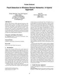
1 Introduction Sensors deployed in the plane are expected to provide us with relevant information depending upon the applications they are used for. Every sensor is equipped with a sensing and transmission device. A sensor can sense targets or other sensors if they are within its sensing range and similarly it can transmit to and receive from a sensor if the two sensors are within their respective transmission ranges. After deployment, sensors form an ad hoc wireless network among themselves by establishing virtual links if two sensors are within each other’s transmission range. It is assumed that the network is connected. Throughout the paper the sensing range of a sensor is equal to its transmission range unless otherwise specified. Consider Figure 1 where a network of six sensors is shown. Sensors u, w are within their transmission range and can sense a target (shown as a rectangle) as it falls in their sensing range. Sensor v can also sense the target but none of u or w is v’s neighbor. After the ad hoc network is formed, sensors begin sensing the environment and depending on the application, such as target tracking, target monitoring, disaster-relief alarm, area coverage, and so on, they cooperate by sending and receiving sensed information among them. The goal of such applications is achieved when relevant and timely information generated from the collaboration of sensors is relayed to a central base station to take appropriate action. As wireless sensors have limited battery power, one critical aspect of such networks is energy consumption which is caused by sensing and transmission activities by individual sensors. The more a sensor engages in sensing and transmitting, the more energy it consumes. Although in most applications a sensor’s energy cannot be replenished, it is generally expected that the sensor will continue to provide information for a long period of time. This raises the 1

v w u

Fig. 1: A sensor network in which three sensors can sense a target which falls in their sensing range.

need to judicially utilize the sensors to obtain required information from the sensing field, since otherwise sensors will quickly drain their energy and be unable to function any longer. Therefore, an algorithm for a wireless sensor network should be energy-efficient in the sense that it ensures the careful use of sensors to reduce energy consumption for sensing and transmission, and at the same time meets the expected standard of quality in the solutions provided by them. If a sensor is engaged in sensing (and /or transmitting) call it active in which case it consumes energy, otherwise the sensor is in the sleep mode in which case it does not loose energy. We use ‘sensor’ and ‘node’ interchangeably in what follows. In this paper we study the target monitoring problem. Given a set of stationary targets T = {t 1 , · · · , tm } and a set V = {v1 , · · · , vn } of sensors, the target monitoring problem asks for generating a large family of subsets of sensors V1 , · · · , Vs called monitoring sets, such that each Vi monitors all targets. The idea is that only one such set is active for any certain period of time and after that time period another set becomes active and so on, thus providing continuous monitoring. However, the objective of this problem is to maximize z = s/k, where k=max u∈V |{i : u ∈ Vi }|. It is assumed that a large number of sensors are deployed in the plane which are in close proximity of the targets, such that for every target there is at least a sensor to monitor it. Considering each i (1 ≤ i ≤ s) as a round, we activate the sensors in Vi in round i to monitor all targets, while all other sensors V \ Vi are put in the energy-efficient sleep mode. Maximizing z, that is, generating a large number of monitoring sets (in other words maximizing s) and at the same time minimizing the number of frequencies of a sensor in these sets (i.e., minimizing k) has a direct impact in prolonging the lifetime of sensor networks. By the lifetime of a sensor network we mean the elapsed time between the deployment of the sensors and the time when the first sensor runs out of energy. By maximizing z, we distribute the monitoring responsibilities among the sensors in a more balanced way. That is, by having a large number of monitoring sets we increase the chance of selecting all sensors in the network in these sets, and by minimizing the number of participations of individual nodes in these sets, we reduce the possibility of selecting the same nodes. Therefore, as nodes in the network are put in the active and the energy-efficient sleep mode alternatively, the lifetime of individual nodes is prolonged and hence the lifetime of the network. Another important aspect of sensor networks is the issue of scalability. Since hundreds or even thousands of sensors may sometimes be deployed to accomplish certain tasks, it is generally expected that the algorithms for such networks be distributed (or more preferably localized) rather than centralized. This is because in a centralized system all sensors have to relay their information (such as id, neighborhood information, etc.) to the central base station which then executes the algorithm and returns the results to the sensors. As this maybe infeasible for large networks, an algorithm of a distributed nature is more acceptable in such cases, which relieves the nodes from sending their information to the central base station. In a distributed system the sensors run the same algorithm individually based on local knowledge of the network. This makes distributed algorithms suitable for large networks. However, a preferred approach is to use a localized system in which each sensor is allowed to know only a constant neighborhood of information to execute its algorithm and make decisions. Define an algorithm as p-localized if each node u is allowed to exchange messages with its neighbors v at most p−hops away and take decisions accordingly based on this information.

2

In order to solve the target monitoring problem we propose a 2-localized algorithm and therefore, a sensor is restricted to know only the 2-hop neighborhood. Another salient feature of the algorithm is that the sensors do not need to know their geographic positions. They only need to know the ids and the connectivity information of their 2-hop neighborhood. The rest of the paper is organized as follows. In Section 2 we describe related work. In Section 3 we provide definitions and assumptions that are used throughout the paper. The localized algorithm is presented in Section 4 and a theoretical analysis of the algorithm follows in Section 5. Experimental results are presented in Section 6. We conclude in Section 7.

2 Related Work Coverage (also called monitoring) has been one of the important topics in sensor networks and has received a lot of attention during the past several years [2, 4, 5, 6, 9, 8, 11, 13, 14]. The main goal of most of the is to devise scheduling algorithms such that individual sensors in the network are assigned rounds which indicate to them during which rounds they will be active and during which rounds they will be in the sleep mode. When a set of sensors monitors a certain area or a target, it is generally possible to monitor the area or the target by a small subset of them. So, it is redundant to make all the sensors active at the same time for the monitoring instead of using the small subset. This observation leads researchers to devise efficient algorithms such that at any time only a small number of sensors are set as active to monitor the area or the targets. In [2] the authors consider the target coverage problem with the goal to minimize energy consumption. Given a set of targets, they propose an energy-efficient centralized scheme to provide coverage to all the targets by disjoint sets of sensors. They divide the sensor set into disjoint subsets and activate each set to perform the covering task. Basically, their main idea is to generate as many disjoint sets of sensors as possible such that each set covers all the targets. However, the algorithm is centralized and does not scale for larger networks. In [12] the authors address the area coverage problem where their algorithm works in two phases. In the first phase the algorithm determines how many different sensors cover the different parts of the monitored area. Like the algorithm in [2], the second phase allocates sensors into mutually independent sets where each set is active at any time to provide the area coverage. The algorithm is also centralized and the authors do not provide any theoretical results regarding the performance of their algorithm. Simulation results show that the algorithm achieves significant power savings (by generating more disjoint sets of sensors) in performing area coverage. The work relevant to ours is [3] where the authors consider the target coverage problem by a set of subsets of sensors while the subsets do not need to be disjoint. They call this the maximum set covers (MSC) problem and present two centralized algorithms, one based on linear programming and the other is a greedy algorithm. They do not provide any theoretical analysis of their algorithms and give simulation results to verify their approaches. In this paper, we consider a target monitoring problem where we focus on generating a large number of monitoring sets and at the same time reducing the number of participations of each node in these generated set. A recent result related to our problem is described in [1], where the authors consider the monitoring schedule problem: Given a set of sensors and a set of targets it is required to find a partition of the sensor set such that each part can monitor all targets. Each part of the partition is used for one unit of time and the goal is to maximize the number of parts in the partition. They present a randomized distributed algorithm which generates at least (1 − ε) ∗ opt (0 < ε < 1) parts, with high probability, where opt is the maximum number of parts in the partition. However, they make the assumption that the sensors must know their geographic positions. The authors also show that by modifying their algorithm they can find a constant approximation factor for the problem and the sensors do not need to know their geographic positions. Our work is related to theirs in the sense that we maximize the number of parts while trying to reduce the use of the same nodes in these parts. Besides, ours is a deterministic algorithm as opposed to their randomized one and the assumption that the sensors know their positions is excluded.

3

3 Model and Definitions We assume that sensors are deployed in the plane and model the underlying sensor network by an undirected graph G = (V, E), where the vertex set V denotes the set of sensors and E represents the links (u, v) ∈ E between two nodes u, v ∈ V if they are within their transmission range, T R. A sensor is equipped with a sensing device that can monitor a target if it falls inside its sensing range, SR. There are a number of reasonable assumptions relating T R and SR and we study two popular ones [1, 7]. In dealing with the target monitoring problem, we consider two situations (i) T R = SR and (ii) T R = 2 ∗ SR. Define the neighbor sets N (u) and N [u] of node u as N (u) = {v|(u, v) ∈ E, u 6= v} and N [u] = N (u) ∪ {u}. By Nf (u) we mean the set of nodes from u which are at most f hops away. For simplicity we use N (u) = N 1 (u). The degree deg(u) of a node is the number of neighbors it has, i.e., deg(u) = |N (u)|. Each node u is identified by a unique index denoted as id(u). When a shortest path between two nodes u, v ∈ V is referred we mean the shortest hop distance between them and denote it by d(u, v). The target set is denoted as T = {t1 , · · · , tm }, where ti is a target. The set of targets monitored by node u is referred to as T (u). For u and t ∈ T (u), Tt (u) represents the set of sensors in N2 [u] that monitors the target t (i.e., Tt (u) = {t|t ∈ T (u) ∩ T (v), v ∈ N2 [u]}). Each node u maintains an ordered pair at each round i (initially i = 1), p i (u) =≺ (cti (u), id(u)) , where the first element cti (u) (also called the counter) denotes the number of monitoring sets in which u has already participated. Initially, ct1 (u) = 0, ∀u ∈ V , and this is incremented by one (cti (u) = cti (u) + 1) each time u participates in some monitoring set. For a subset X, and two nodes u, v ∈ X, we say that node u is lexicographically smaller than node v at round i if pi (u) < pi (v), i.e., either cti (u) < cti (v) or cti (u) = cti (v) and id(u) < id(v). The rank of node u with respect to X, denoted by r(X(u)), is the index of u in the lexicographically sorted (ascending order) nodes of X.

3.1 Problem Formulation We formulate the target monitoring problem in the following way. Given a set of m targets T = {t 1 , · · · , tm } and a set of n sensors V = {v1 , · · · , vn } (both) randomly deployed in the plane such that for each target in T there is at least one sensor that monitors it, we would like to find a family V of subsets V 1 , · · · , Vs such that i) ∀i, Vi monitors all targets in T , ii) z = s/k is maximized, where k=maxvj ∈V |{i : vj ∈ Vi }|.

4 The Algorithm In this section we present a 2-localized algorithm for the target monitoring problem and discuss some problems related to the myopic view of localization. We assume that the transmission range T R is equal to the sensing range SR. As individual nodes execute the same algorithm, we describe what happens to an arbitrary node u in the network. Our algorithm works in rounds starting from round 1. At the first round (i = 1), node u forms its monitored target list T (u) by sensing (or monitoring) the targets in its sensing range. Then u sends two items to all its neighbors which are at most 2-hops away. It sends its list T (u) and an ordered pair pi (u) =≺ (cti (u), id(u))  to v ∈ N2 (u). Note that initially ct1 (u) = 0. Similarly u receives such information (T (v) and pi (v)) from all its neighbors v ∈ N2 (u). Thus u knows the targets that are monitored by its one and two hop neighbors. After obtaining T (v) and pi (v) from all its one and two hop neighbors, u forms the set Ta (u) for each of its monitored target a ∈ T (u) (recall that Ta (u) = {a|a ∈ T (u) ∩ T (v), v ∈ N2 [u]}). In other words, the set Ta (u) refers to the sensors monitoring target a that are at most 2-hops away from u. Then for each T a (u), u computes its rank r(Ta (u)) in this round. If u is the smallest ranked node in any Ta (u), then it becomes active to monitor a, otherwise it goes into the sleep mode. According to the notation, all active nodes in round i are represented by V i which monitor all the targets. For example, if sensors u1 , u2 , u3 (assume the subscript denotes the respective id) monitor target b (see Figure 2) then |Tb (u1 )| = 3. At round 1, u1 becomes active by being the smallest ranked node for monitoring b while the other two nodes can go into the sleep mode, then at rounds 2 and 3, u 2 and u3 take their turn to be active

4

by becoming the smallest ranked node, respectively. Thus the monitoring sets in round 1,2, and 3 are V 1 = {u1 }, V2 = {u2 } and V3 = {u3 }, respectively. If u becomes active in round i then its counter is incremented by one (ct i+1 (u) = cti (u) + 1), otherwise the counter value remains the same. Node u then sends its pi+1 (u) =≺ (cti+1 (u), id(u))  to, and receives pi+1 (v) from v ∈ N2 (u) and a new round i + 1 begins. As before u computes its rank (since p i+1 (.) values are updated) for each target a ∈ T (u). The smallest ranked node for a target a becomes active and starts monitoring a. All smallest ranked nodes in the network form the monitoring set Vi+1 which monitors all targets in T and so on. The algorithm is given in Figure 3.

4.1 A Problem with Locality In general, it is assumed that sensors which are in close proximity in the plane sense or observe the same data due to the spatial correlation. For a subset Xt of nodes that monitor the same target t in some round, it is supposed that the nodes will be in close proximity. However, the nodes in Xt , although they monitor the same target, can have arbitrarily long hop distance between each other, while the Euclidean distance maybe slightly more than their transmission range. We call this situation the Locality Effect, where the monitoring nodes for a certain target do not know about each other about their monitoring. In Figure 1, the Euclidean distance between u and v is T R + ε (recall that 0 < ε < 1) and they both monitor the same target (shown as a rectangle) whereas their shortest path d(u, v) (in terms of hop distances) can be arbitrarily long.

u2

u1 b

u3

Fig. 2: Nodes u1 , u2 , and u3 monitor target b and the monitoring sets are Vi = {ui }, ∀i

5 Theoretical Analysis In this section we give an overview of the theoretical analysis of the algorithm. Consider a target t ∈ T and let X t be the set of sensors that monitors it in some round. For any node u ∈ X t , u knows only whether other nodes, which are within its 2-hop neighborhood (i.e., N2 [u]), can monitor t and therefore chooses exactly one among N 2 ([u]) for the monitoring. However, due to the locality effect there can be two nodes u, v ∈ X t such that v ∈ / N2 (u) and both u and v monitor t and u does not have any clue about v. We would like to determine an upper bound on how many sensors can monitor a target while none of them is aware of the other. First, we have the following simple observation from our algorithm. Observation 5.1 The set Vi of all active nodes monitors all targets in T at round i. As one of the main results, we show that at any round at most five sensors can simultaneously monitor a target, none of which is within the 2-hop neighborhood of the other. In the following, we assume that T R = SR. Lemma 5.2 For any target t ∈ T , at most five sensors are set as active.

5

Input: A connected graph G = (V, E) and a set of targets T such that each target is monitored by at least one sensor. Output: A family of subsets of sensors V1 , · · · , Vs such that each Vi monitors all targets in T . 1: i = 1 2: Broadcast pi (u) and T (u) to v ∈ N2 (u) 3: Receive pi (v) and T (v) from v ∈ N2 (u) 4: Compute Ta (u) = {a|a ∈ T (u) ∩ T (v), v ∈ N2 (u)}, ∀a ∈ T (u) 5: /*Ta (u) represents the set of sensors that monitor a*/ 6: For each round i 7: Compute rank r(Ta (u)), ∀a ∈ T (u) 8: If ∃a ∈ T (u) such that 9: r(Ta (u)) < r(Ta (v)), v ∈ N2 (u) Then 10: /*Selects the smallest ranked node for each target*/ 11: u becomes active 12: Endif 13: i = i + 1 14: If u is active Then 16: cti (u) = cti−1 (u) + 1 17: Endif 18: If cti (u) 6= cti−1 (u) Then 19: Send pi (u) to v ∈ N2 (u) 20: Endif 21: Receive pi (v) from v ∈ N2 (u) 22: Endfor Fig. 3: A 2-Localized algorithm for the target monitoring problem Proof Assume Xt to be the set of sensors that monitors a target t ∈ T in some round. Suppose for the sake of contradiction that |Xt | > 5 and no two nodes u, v ∈ Xt are within the 2-hop neighborhood of the other. As t is monitored by all sensors in Xt , the Euclidean distance between t and any node w ∈ Xt must be at most SR. Consider a disk D centered at t with radius equal to SR. Therefore, all the nodes in X t must be within the disk D. Since |Xt | > 5 and nodes of Xt are in D, there will be at least two nodes u0 , v 0 ∈ Xt whose Euclidean distance must be smaller than T R (we can consider T R the radius of D instead of SR, since SR = T R). Then u 0 and v 0 are direct neighbors to each other, a contradiction. A tight example of the above lemma is shown in Figure 4, where five sensors are put on the vertices of a regular pentagon with side T R + ε. They can all monitor any target t in the striped region S which is the intersection of their respective sensing disks. Note that for any ui , ui ∈ / N2 [uj ] (i 6= j and i, j ∈ {1, 2, 3, 4, 5}). Then we derive the corollary from the above lemma. Corollary 5.3 If Vi∗ denotes the minimal set of sensors monitoring targets at round i, then |V i | ≤ 5m|Vi∗ |, where m = |T | is the number of targets given. An implication of the above corollary is that if we have a constant number of targets (|T | = m ≤ c, c is a constant) to be monitored then, at any round, the number of sensors becomes active by the algorithm is within a constant factor of the optimal, i.e., |Vi | ≤ 5c|Vi∗ |. Now we show how the algorithm performs towards maximizing the value of z = s/k. First we need some notation. Let X1 , X2 , · · · , Xm be the subsets of sensors (Xi ⊆ V , 1 ≤ i ≤ m) that monitor the targets t1 , t2 , · · · , tm , respectively, in some round. Let Xp be the minimum cardinality subset among all Xi ’s (ties are broken arbitrarily). 6

u5

u1

u4

u2

u3

Fig. 4: For a target in the striped region (intersection of the five disks) we set as active at most five sensors whereas only one sensor suffices.

Now we divide each Xi (Xi monitors target i) in the following way. Due to the locality effect we can have at most five subsets Xi (i1 ), Xi (i2 ), Xi (i3 ), Xi (i4 ) and Xi (i5 ) of Xi (i.e., Xi (ia ) ⊆ Xi , 1 ≤ a ≤ 5, 1 ≤ i ≤ m) such that no node in one subset knows whether any nodes in other subsets are monitoring i. In other words, there is no node u ∈ Xi (ia ) such that v ∈ Xi (ib ), a 6= b and v ∈ N2 [u]. Let X ∗ =min1≤i≤m,1≤a≤5 |Xi (ia )|. Note that |X ∗ | ≥ 1. Denote by zopt the optimal value of z and zopt > 0, that is, zopt ≥ z = s/k for all possible values of s and k. If zalg denotes the value of z obtained by our algorithm then we have the following lemma: Lemma 5.4 zopt = |Xp | and zalg ≥ 1. Hence zopt is at most |Xp | times the value of zalg . Proof First we derive the value of zopt . In order to compute the value zopt , notice that there can be |Xp | monitoring sets V1 , V2 , · · · , V|Xp | such that each node in Xp can participate in these monitoring sets exactly once. It is easy to see that for the optimal algorithm to generate the |Xp | + 1-st monitoring set, V|Xp |+1 , there will be at least one node in Xp such that the number of participations of the node in V1 , V2 , · · · , V|Xp | , V|Xp |+1 is at least two (because of the Pigeonhole Principle). Thus zopt = s/k = |Xp |, where s = |Xp | (i.e., |Xp | monitoring sets V1 , V2 , · · · , V|Xp | ) and k = 1. We now analyze the behavior of the algorithm to find zalg . With each node participating exactly once, the algorithm can generate X ∗ monitoring sets V1 , V2 , · · · , VX ∗ , since only one node is selected in each iteration from X ∗ . Hence zalg ≥ |X ∗ | ≥ 1. Hence zopt is at most |Xp | times the value of zalg .

5.1 T R = 2 ∗ SR In this section we assume that the transmission range of a sensor is twice its sensing range, T R = 2 ∗ SR. In the previous subsection it is shown that we can achieve a good approximation factor (a constant factor) for the size of each of the monitoring sets. However, when the number of targets is a constant, the approximation factor is much worse towards minimizing the value of k. This is because of the very limited information of the 2-hop neighborhood available to individual sensors and we assumed that the transmission range is equal to the sensing range of a sensor. Here we investigate whether the value of k can be improved by assuming T R = 2 ∗ SR. This is a very reasonable assumption in the context of coverage (monitoring) problems in sensor networks [7]. However, we use this assumption and obtain some useful results for the target monitoring problem. Observation 5.5 Let node u ∈ V monitor T (u) ⊆ T targets. If there is a node v ∈ V , v 6= u such that T (u)∩T (v) 6= φ, then v ∈ N (u).

7

Proof Suppose for contradiction, v ∈ / N (u). Since T (u) ∩ T (v) 6= φ, that means v can monitor a target which u can monitor. In this case the Euclidean distance between u and v can be at most twice their sensing range (see Figure 5, where dotted and solid circles represent the transmission and the sensing ranges, respectively) contradicting the fact that v is not a direct neighbor of u.

u

v object

Fig. 5: If T (u) ∩ T (v) 6= φ then v ∈ N (u). The above observation implies that if u monitors t then u knows exactly which other nodes are also monitoring t and moreover, all such nodes are u’s direct neighbors. Lemma 5.6 Under the assumption that T R = 2 ∗ SR, for any target t ∈ T , exactly one sensor is set as active. Proof The proof is similar to the proof of Lemma 5.2. Consider a target t ∈ T and let X t be the subset of sensors that monitors it. There is no locality effect as evident from Observation 5.5. So each node in X t knows whether all other nodes in Xt are monitoring t. Hence the node with the smallest rank in Xt will be active to monitor t. We obtain the following directly from the above lemma: Corollary 5.7 If Vi∗ denotes the minimal set of sensors monitoring targets at round i, then |V i | ≤ m ∗ |Vi∗ |, where m = |T | is the number of targets given. As before, if the number of targets is a constant, the number of active sensors at each round will be within a constant factor of the optimal number of active sensors, |Vi | ≤ c0 ∗ |Vi∗ |, where c0 is a constant. In the following, we show that our algorithm obtains optimal results in special instances. Let X 1 , X2 , · · · , Xm be the subsets of sensors that monitor the targets t1 , t2 , · · · , tm , respectively, where Xi ⊆ V in some round. Let Xp be the minimum cardinality subset among all Xi ’s (ties are broken arbitrarily). If Xi ∩ Xj = φ, i 6= j and 1 ≤ i, j ≤ m, that is, a sensor exactly monitors one target, then we have the following lemma. Lemma 5.8 With the above assumption and T R = 2 ∗ SR, we have z alg = zopt Proof Let Xp = {u1 , u2 , · · · , u|Xp | } denote the subset of sensors that monitor p (recall that Xp has minimum cardinality among |Xi |’s). The optimal algorithm can produce |Xp | monitoring sets V1 , V2 , · · · V|Xp | with each node in Xp participating exactly once. Since Xp has the smallest cardinality, for the optimal algorithm to produce the next monitoring set V|Xp |+1 , at least one of the nodes in Xp must be selected in V|Xp |+1 . So, zopt = |Xp |/1 ≥ (|Xp |+1)/2. Now we see how the algorithm behaves towards finding zalg . Since there is no locality effect (all nodes u1 , u2 , · · · , u|Xp | are aware of each other about monitoring p), the algorithm sets as active exactly one node from X p (say node uj is selected in some round). Since Xp ∩ Xi = φ, for i 6= p and 1 ≤ i ≤ Xm , no other nodes from Xp will be selected (active) in that round. Therefore, at any round exactly one node is set as active from X p and hence we have V1 , V2 , · · · V|Xp | monitoring sets. Now we show that any node uj ∈ Xp is exactly used once in V1 , V2 , · · · V|Xp | monitoring sets. 8

Suppose for contradiction that a node uj is used in monitoring sets Vr and Vw , where 1 ≤ r, w ≤ |Xp | and r < w. After being selected first in Vr , uj ’s ct(uj ) value is increased by one. If uj is selected (from Xp ) again in Vw , that means its rank is smaller than other nodes in Xp . Since w ≤ |Xp | and exactly one node is selected from Xp , there is at least some node in Xp which has not been selected in previous monitoring sets V1 , V2 , · · · , Vw0