Techniques for Improving Vision and Locomotion on the ... - CiteSeerX

Techniques for Improving Vision and Locomotion on the Sony AIBO Robot Michael J. Quinlan, Stephan K. Chalup and Richard H. Middleton∗ School of Electrical Engineering & Computer Science The University of Newcastle, Callaghan 2308, Australia {mquinlan,chalup,rick}@eecs.newcastle.edu.au

Abstract The restricted setting and uniformly prescribed hardware of the Sony Legged League of RoboCup provide an environment for testing algorithms on autonomous robots with a view towards possible applications in real world situations. In this study we show how two techniques - Support Vector Machines and Hill Climbing - can be applied to problems faced by the robots in this league. We use Support Vector Machines to perform collision detection and also to assist the process of color classification, while a Hill Climbing algorithm is employed to improve straight line walking speed through walk parameter optimisation.

1

Introduction

Sony AIBO robots are currently used in the Legged League of RoboCup. The OPEN-R software libraries are designed for use with modular robot architectures and are already becoming a standard for a larger class of future robots [OPEN-R, 2003]. OPEN-R is free and the robots are available for purchase in many countries and via the internet. However programming the robots to perform certain tasks or show adaptive behavior remains a challenge even for experts. One reason for this is their limited hardware capabilities. Traditionally hard coding of expert knowledge and handtuning of parameters have been preferred over the use of learning algorithms on the robot. Application of the latter is often restricted to simulations which are able to support training or tuning of the real world robot parameters. However, often the gap between simulation and the real world is very wide. This often renders the transfer of training results from the simulated to the real robot useless. In this article we report how we are able to improve the robots’ performance with respect to colour classification, collision detection and straight line walking speed using two types of machine learning algorithm. ∗

http://www.robots.newcastle.edu.au

2

Hardware and Environment

Before discussing the machine learning algorithms we briefly review the hardware and environment for robot soccer.

2.1

Sony AIBO

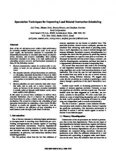
The legged league in 2003 prescribed the use of Sony AIBO entertainment robots (Figure 1), models ERS-210 or the newer ERS-210A. Both have an internal 64-bit RISC processor with clock speeds of 192MHz and 384MHz, respectively. The robots are programmed in a C++ software environment using the Sony’s OPEN-R software development kit. The dimensions of the robot (width × height × length) are 154 mm × 266 mm × 274 mm (not including the tail and ears) and the mass is approximately 1.4 kg. The use of servos gives the robot 20 degrees of freedom (DOF): Neck 3DOF (pan, tilt, and roll), Ear 1DOF x 2, Chin 1DOF, Legs 3DOF (Abductor, Rotator, Knee) x 4 and Tail 2DOF (Up-Down, Left-Right).

Figure 1: Sony AIBOs on the RoboCup Legged League field.

2.2

RoboCup Legged League

Soccer matches take place on a green carpeted field with internal dimensions of 270 cm × 420 cm, surrounded by a 10 cm high sloped white wall. Localisation is aided by six beacons uniquely identifiable by a specific colour pattern

which are placed around the field. Two goals, a blue and a yellow, are positioned on opposite ends of the field. Currently the ball used is orange plastic and of a suitable size to be easily moved around by the robots. The games consist of two ten minute halves under rules imposed by independent referees.

To construct the optimal hyperplane one solves a constrained optimisation problem by introducing Lagrange multipliers αi ≥ 0 and a Lagrangian L(w, b, α) =

3 Techniques and Tasks

` X 1 kwk2 − αi (yi · ((xi · w) + b) − 1). (3) 2 i=1

In this section we will give a brief overview of the theory behind Support Vector Machines (SVMs) and Hill Climbing. We will show how we applied variations of these techniques to the tasks of colour classification, collision detection and walk parameter optimisation.

L has to be minimised with respect to the primal variables w and b and maximised with respect to the dual variables αi . The derivatives of L with respect to these primal variables leads to ` X αi yi = 0 (4)

3.1 Support Vector Machines

and

i=1

The origins of the Support Vector Machine can be traced to Vapnik’s work on Statistical Learning Theory [Vapnik and Lerner, 1963; Vapnik, 1979; 1998]. It wasn’t until the early 1990’s that it was further developed [Boser et al., 1992; Cortes and Vapnik, 1995; Vapnik, 1995] and commonly employed for classification tasks such as handwriting or face recognition. The SVM was first developed for two-class classification, the simplest version being known as a maximum margin classifier (Figure 2). This version only works on linearly separable data by selecting the hyperplane that separates the two classes by the largest margin.

w=

` X

αi yi xi

(5)

i=1

Substituting (4) and (5) into L gives us a dual problem, ` X

` 1 X max αi − αi αj yi yj (xi · xj ) 2 i,j=1 i=1

(6)

subject to αi ≤ 0, i = 1, ..., `, and

` X

αi yi = 0.

i=i

This results in the following decision function for the hyperplane ` X f (x) = sgn( yi αi · (x · xi ) + b)

(7)

i=1

To build a non-linear SVM, one maps the input variable into a high dimensional (possibly infinite) dot product feature space that is hidden from both the input and the output. We then construct an optimal hyperplane to separate the features discovered in the feature space. Since (6) and (7) only require the evaluation of dot products, by replacing xi · xj with a Mercer kernel k(xi , xj )=Φ(xi ) · Φ(xj ) the algorithm will find a hyperplane in a high dimensional space with very little impact on run time. Some commonly used kernels are k(xi , xj ) =

Figure 2: Maximal Margin Classifier: Separating hyperplane where the shaded inputs are support vectors. The training data is labelled {xi , yi }, i = 1, ..., `, yi ∈ {−1, 1}, xi ∈ Rn . If you consider the class of hyperplane (w · x) + b = 0 w ∈ Rn , b ∈ R

Radial Basis F unction = P olynomial =

(1)

where w is a weight vector and b a threshold, there exists a unique optimal hyperplane with the maximum margin given by n

max min{kx − xi k : x ∈ R , (w · x) + b = 0}. w,b

e−γkxi −xj k (xi · xj )d

2

We now get a generalised version of the decision in function (7) f (x) = sgn(

(2)

` X i=1

2

yi αi · k(x, xi ) + b)

(8)

Overlapping data (i.e. noisy data) can be handled by using a soft margin classifier, this is achieved by adding slack variables. By solving with relaxed constraints a classifier can be constructed that can allows you to maximise the capacity while minimising the number of training errors. Enhancements to the SVM algorithm allows for multi-class classification along with one-class classification. The remainder of the paper focuses on a one-class SVM technique.

An implementation of this approach is available in the LIBSVM library [Chang and Lin, 2001]. It solves a scaled version of (9): 1X αi αj k(xi , xj ) (12) min α 2 ij subject to 0 ≤ αi ≤ 1 and

X

αi = ν`

i

One-class SVM

For our applications we use a RBF kernel with parameter γ 2 in the form k(xi , xj ) = e−γkxi −xj k .

An approach to one-class SVM classification was proposed by Sch¨olkpof et al. [Sch¨olkopf et al., 2001]. Their strategy is to map data into the feature space corresponding to the kernel function and to separate them from the origin with maximum margin. This implies the construction of a hyperplane such that w · Φ(xi ) − b ≥ 0 (Figure 3). The result is a function f

Colour Classification The vision system for most teams consists of four main tasks, Colour Classification, Run Length Encoding, Blob Formation and Object Recognition The classification process takes the image from the camera in a YUV bitmap format [Shapiro and Stockman, 2001]. Each pixel in the image is assigned a colour label (i.e. ball orange, beacon pink etc.) based on its YUV values. A lookup table (LUT) is used to determine which YUV values correspond to which colour labels. The critical stage is the initial generation of the LUT. Since the robot is extremely reliant on colour for object detection a new LUT has to be generated with any change in lighting conditions. Currently this is a manual task which requires a human to take hundreds of images and assign a colour label on a pixel-by-pixel basis. Using this method each LUT can take hours to create, yet it will still contain holes and classification errors. The classification functions we seek take data that has to produce sets X k = © k been3 manually clustered ª xi ∈ R ; i = 1, ..., Nk of colour space data for each object colour k. Each X k corresponds to sets of colour values in the YUV space corresponding to one of the known colour labels. The previous method involved converting the existing LUT values from YUV to the HSI colour space [Shapiro and Stockman, 2001] and fitting an ellipsoid, E, which can be represented by the quadratic form: n o T E (x0 , Q) = x ∈ R3 : (x − x0 ) Q−1 (x − x0 ) ≤ 1 (13) where x0 is the centre of the ellipsoid, and the size, orientation and shape of the ellipsoid are contained in the positive definite symmetric matrix Q = QT > 0 ∈ R3×3 . Note that this definition of the shape can be alternatively represented by the linear matrix inequality (LMI): · ¸ Q (xi − x0 ) xi ∈ E = ≥0 (14) T (xi − x0 ) 1

Figure 3: One-class SVM: The boundary produced by the one-clss SVM contains only the input points. that returns the value +1 in the region containing most of the data points and -1 elsewhere. Assuming the use of an Radial Basis Function (RBF) kernel where ν approximates the fraction of outliers and support vectors and i, j ∈ {1, ..., `}, we are presented with the dual problem: min

1X αi αj k(xi , xj ) 2 ij

0 ≤ αi ≤

X 1 and αi = 1 ν` i

α

(9)

subject to

b can be found by the fact that for any such αi , a corresponding pattern xi satisfies: b=

X

αj k(xj , xi )

(10)

j

The resulting decision function f (the support of the distribution) is: X f (x) = sign( αi k(xi , x) − b) (11)

The LMI (14) is linear in the unknowns Q and x0 and this therefore leads to the convex optimisation:

i

3

(Q, x0 ) =

argmin {tr(Q)} Q = QT > 0, x0 : (14) is true for i = 1..Nk

The second situation in which we use the one-class SVM is on a completed LUT. Either all colours in the table can be trained (i.e. updating of an old table) or an individual colour is trained due to an initial classification error. This procedure can be performed either on the robot or a remote computer.

(15)

Note that minimising the trace of Q (tr(Q)) is the same as minimising the sum of the diagonal elements of Q which is the same as minimising the sum of the squares of the lengths of the principal axes of the ellipsoid. The ellipsoidal shape defined in (13) has the disadvantage of restricting the shape of possible regions in the colour space. However, it does have the advantage of having a simple representation and a convex shape. Before the ellipsoid can be fitted, potential outliers and duplicate points were identified and removed. The removal of outliers is important in avoiding too large a region. Duplicate points were removed, since these increase computations without adding any information. In the new solution an individual one-class SVM is created for each colour, with X k being used as the training data (each element in the set is scaled between -1 and 1). By training with an extremely low ν and a large γ the boundary formed by the decision function approximates the region that contains the majority (1-ν) of the points in X k . In addition the SVM has the advantage of simultaneously removing the outliers that occur during manual classification. The new colour set is constructed by attempting to classify every point in the YUV space (643 elements). All points that return a value of +1 are inside the region and therefore deemed to be of colour k. Constructing an independent SVM for each colour gives us the greatest flexibility in attempting to create an optimal classification for each colour. By applying a simple priority system to colours (e.g. ball orange over beacon pink) potential overlaps are avoided. The SVM can be used in two situations during the colour classification procedure. Firstly during the construction of a new LUT where it can be applied to increase the speed of classification. By lowering γ while the number of training points is low, a rough estimation of the final shape can be obtained. By continuing the manual classification and increasing γ a closer approximation to the area containing the training data is obtained (Figure 4). In this manner a continually improving LUT can be constructed until it is deemed adequate. An extreme example of this application is during the set-up phase at a competition. In the past when we arrived at a new venue all system testing was delayed until the generation of a LUT. Of critical importance is testing the locomotion engine on the new carpet and in particular ball chasing. The task of ball chasing relies on the classification of ball orange. Thus a method of quickly but roughly classifying orange is valuable. By manually classifying a few images of the ball and then training the SVM with γ < 0, a sphere containing all possible values for the ball is generated.

Results First an individual LUT was generated for each image in a test set. Each of these LUTs is designed to provide a near optimal result for its corresponding image. This provides us with a reference so we can compare LUTs for a measure of accuracy. The LUTs were compared over 60 images, which equates to 1520640 individual pixel comparisons. Lookup Table Hand generated ν=0.025 and γ=10 ν=0.025 and γ=250 ν=0.025 and γ=500 ν=0.025 and γ=1000

Errors 144098 153060 117652 126840 135778

% Error 9.48 10.07 7.74 8.34 8.93

Experimental results indicate that ν = 0.025 and γ = 250 provide excellent results on a previously constructed LUT. An example image can be seen in Figure 5. The most evident change can be seen in the classification of the colour white due to a 250% increase in white entries in the LUT. Collision Detection For collision detection the one-class SVM is employed as a novelty detection mechanism [Marsland, 2003]. In our implementation each training point is a vector containing thirteen elements. These include five walk parameters, stepFrequency, backStrideLength, turn, strafe and timeParameter along with a sensor reading from the abductor and rotator joints on each of the four legs. Upon training the SVMs decision function will return +1 for all values that relate to a “normal” step, and -1 for all steps that contain a fault. Speed is of the greatest importance in the RoboCup domain. For this reason a collision detection system must attempt to minimise the generation of false-positives (detecting a collision that we deemed not to have happened) while still finding a high percentage of actual collisions. Low falsepositives are achieved by keeping the kernel parameter γ high but this has the side effect of lowering the generalisation to the data set, which results in the need for an increased number of training points. In a real world robotic system the need for more training points greatly increases the training time and in-turn the wear on the machinery. The previous method, described in [Quinlan et al., 2003], for collision detection involves observing a joint position substantially differing from its expected value. In our case an empirical study found two standard deviations to be a practical measure, see Figure 6. Initially we would have considered a collision to have occurred if a single error is found, but further investigation has shown that finding multiple errors (in 4

Figure 4: Colour Classification: A) Points manually classified at white. B) Ellipsoid fitted to these white points. C) Result of the one-class SVM technique, ν=0.025 and γ=10. D) Result of the one-class SVM technique, ν=0.025 and γ=250.

Figure 5: Image Comparison: The left image is classified with the original LUT and the image on the right is the using the updated LUT. Black indicates a pixel that has been classified as unknown.

most cases three) in quick succession is necessary to warrant a warning that can be acted upon by the robot’s behaviour system. One drawback of this method is that it relied on domain knowledge to arrive at two standard deviations. In addition it required considerable storage space to hold the table of means and standard deviations for each parameter combination. The previous statistical method had the advantage of extremely low computational expense, in fact it was a table look

up. The trade-off is increased space, this method required the allocation of approximately 6MB of memory during both the training and detection stages. Conversely the SVM approach requires only about 1MB of memory during the detection phase, but this comes at the side effect of increased computation. Since the SVM approach was capable of running without reducing the frame rate, the extra memory could now be used for other applications.

5

a brief description of the 13 parameters in our system (front and back are described together) Front/Back Height - Height of front/back hip above the ground (mm) Front/Back Sideways Offset - Distance measured from the shoulder of the paw to the side (mm) Front/Back Forward Offset - Distance of the paw from the shoulder to the front (mm) Front/Back Stride Height - The maximum height the paw will be lifted of the ground (mm) Step Frequency - Number of steps per second the robot will take Figure 6: Rear Right Rotator for a forwards walking boundary collision on both front legs, front right leg hitting first. The bold line shows the path of a collided motion. The dotted line represents the mean “normal” path of the joint (that is, during unobstructed motion), with the error bars indicating two standard deviations above and below.

Front/Back Stride Length - Length of step (mm) Turn - The angle the robot should turn (counter clockwise) during the step (degrees) Strafe - Distance to the left the robot should move during the step (mm) The robot’s legs each follow a trajectory (or locus) in 3dimensional coordinate space. The current system only defines a locus with vertical and forward components. The locus is rotated about the vertical axis to allow the robot to turn. Various locus shapes have been tested, including rectangular, elliptical and trapezoidal. Although the trapezoidal locus has provided us with the best results in the past, it is not clear that this shape is optimal. With this in mind, a system to easily allow arbitrarily complex locus shapes has been developed. For reasons of efficiency and flexibility, the algorithm for defining and following an arbitrary locus is quite involved. More precisely, the arbitrary locus must be deformable to allow the walk parameters to easily control the robot’s motion and maintain the advantages of a highly parameterised motion engine. Additionally, there is only a very limited amount of processor time available for locomotion, meaning that time consuming operations can only be performed occasionally. An arbitrary locus is defined by an arbitrary number of ‘critical points’ that, when joined together by straight lines, represent the desired locus shape. The critical points need not be a fixed distance apart. For a rectangular locus, the critical points would be the four corners. Only the shape of the locus is relevant, as its size is scaled later. We would argue that using straight lines is much less of a limitation than it seems, as an arc can easily be represented by using several points. Furthermore, there is little point in using spline curves as the robot’s joint motors tend to smooth out the leg motion anyway. When a new set of walk parameters is received by the locomotion engine, a number of steps must be performed in sequence to prepare an arbitrary locus for use. Firstly, the critical points must be deformed to account for walk parameters. For example, the critical points may have to be stretched for a large stride length, or compressed for a small stride height.

Results Results were gathered in a two step process. First was a test in which the robot was placed in a situation where no collisions would occur - this test was designed to find false positives (detecting a collision that we deemed not to have happened). In the second test we placed the robot directly in front of the field boundary to test the success rate of detecting a collision. It should be noted that there is a level of human interpretation (and therefore human error) in the gathering of data: The output of the system is compared against what we perceived to have occurred. Therefore if the system did not trigger an expected fault this may be the result of an incorrect human assumption. For the detection of collisions while walking forwards, the statistical method produced false positives in fewer than 1% of steps. About 98% of collisions were detected. In terms of accuracy the SVM approach slightly outperformed the original statistical method for similar collisions.

3.2

Hill Climbing for Walk Parameter Optimisation

The majority of teams in the legged league use some form of omnidirectional parameterised walk based on the work of [Hengst et al., 2002]. The end of each paw is commanded to follow a trajectory with inverse kinematics used to calculate the joint angles required to achieve the positions. Commonly referred to as “PWalk” the original version followed a rectangular trajectory and contained 8 parameters that effect the stance of the robot and 4 parameters that control size and direction of each step. Our version has an additional control parameter because we separated the forward parameter into front and back stride lengths. The following is 6

This is a simple matter of scaling the coordinates of the critical points so the shape they define is of the appropriate dimensions. The next - and final - step before walking can commence is interpolation. This task is performed prior to walking primarily for reasons of efficiency. The algorithm linearly traverses the deformed critical points and defines new points at (small) fixed intervals. These evenly spaced points allow the walk engine to efficiently control the timing of the locus traversal when actually walking. Simply put, the walk engine must be able to very efficiently calculate the exact position of each leg in 3-dimensional space at any given time during a step. Currently optimising the robots walk is done by hand manipulation of the parameters. The optimal parameter vector will differ for each surface and each trajectory. Fixing problems (i.e. slip) may involve the change of one or all of the parameters, thus the parameter space is too large to be covered by a human. The addition of an arbitrary locus serves to further increase the size of the parameter vector. Because we are dealing with a real world robot where each episode may take up to 30 seconds we need a solution with a steep learning curve.

human derived time of 382 (24.87cm/s). Although this example has a lowest time of 315 the parameter set that achieved this time is unreliable. The lowest repeatable time for a trapezoidal trajectory is 327.69 with a standard deviation of 4.69 (28.99 cm/s ± 0.4). 550

500

Time

450

400

350

300

0

10

20

30

40

50

60

70

Episodes

Figure 7: Results of EHCLS with a trapezoidal locus. The horizontal line indicates the initial human derived time of 382. The second set of experiments involved learning both the walk parameters and the critical points for an arbitrary locus shape. We decided on 10 critical points (each critical point consists of an x,y pair). With different sets of critical points for the front and back legs we now have an additional 40 parameters to tune and thus a θ of size 51.

Evolutionary Hill Climbing with Line Search A version of Hill Climbing [Chalup and Maire, 1999] was chosen because it can provide good results in parameter optimisation problems. We have chosen to use an Evolutionary Hill Climbing with Line Search (EHCLS) algorithm, which should provide a reasonably quick learning time. The walk engine is determined by a vector θ containing the set of 11 walk parameters (turn and strafe are excluded from the learning) and the critical points defining an arbitrary locus shape. Each parameter is randomly set to an initial value; For our task we make sure the initial vector is adequate (i.e. it is capable of walking). In our experiment one episode is to be defined as two runs of approximately 190cm each with time being the number of vision frames processed during the episode. Both the number of runs and distance can be modified to suit the environment. The exact distance travelled can’t be guaranteed as the robot uses it own vision system to trigger the completion of a run.

400

390

380

370

Time

360

350

340

330

320

310

300

0

10

20

30

40 50 Episodes

60

70

80

90

Figure 8: Results of EHCLS with an arbitrary locus shape. The horizontal line indicates the initial human derived time of 382.

Results Initially we ran the experiment on each of the three static trajectories - rectangular, ellipsoid and trapezoidal. With human optimisations we have found that the original rectangular trajectory was the slowest followed by the ellipsoid and then the trapezoidal trajectory. In these experiments θ only contained the walk parameters (excluding strafe and turn) and therefore had a size of 11. The results show that EHCLS was capable of improving on the best parameter set for each trajectory, again the trapezoidal was the fastest followed by ellipsoid and rectangular. An example training exercise for a trapezoidal trajectory is shown in Figure 7. The horizontal line indicates the initial

Results for training with arbitrary locus shape is shown in Figure 8. The fastest repeatable time gained by the arbitrary locus is 320.51 with a standard deviation of 8.01 (29.65 cm/s ± 0.7) with the locus shape shown in 9. It should be noted that the θ that produced these results is a direct descendant of the θ that produced the best trapezoidal time. Also the initial critical points formed a trapezoid. Figure 10 shows the result of learning when the initial critical locus was substantially different to a trapezoid. This example resulted in a best time of 343 (27.70 cm/s). Further 7

References [Boser et al., 1992] B. E. Boser, I. M. Guyon, and V. N. Vapnik. A training algorithm for optimal margin classifiers. In D. Haussler, editor, Proceedings of the 5th Annual ACM Workshop on Computational Learning Theory, pages 144– 152, Pittsburgh, PA, July 1992. ACM Press.

Figure 9: Arbitrary Locus. The red (right) shows the locus shape for the front legs. The blue (lef t) shows the locus shape for the back legs.

[Chalup and Maire, 1999] Stephan Chalup and Frederic. Maire. A study on hill climbing algorithms for neural network training. In Proceeeding of the 1999 Congress on Evolutionary Computation (CEC’99), pages 2014–2021, 1999.

experiments with different locus shape have been unable to improve on the time set by the arbitrary locus shape derived from a trapezoid.

[Chang and Lin, 2001] Chih-Chung Chang and ChihJen Lin. LIBSVM: a library for support vector machines, 2001. Software available at http://www.csie.ntu.edu.tw/˜cjlin/libsvm.

420

400

[Cortes and Vapnik, 1995] C. Cortes and V. Vapnik. Support vector networks. Machine Learning, 20:273 – 297, 1995.

Time

380

[Hengst et al., 2002] B. Hengst, S.B. Pham, D. Ibbotson, and C. Sammut. Omnidirectional locomotion for quadruped robots. RoboCup 2001: Robot Soccer World Cup V, pages 368–373, 2002.

360

340

320

300

0

5

10

15

20

25

30

[Marsland, 2003] Stephen Marsland. Novelty detection in learning systems. Neural Computing Surveys, 3:157–195, 2003.

35

Episodes

[OPEN-R, 2003] Sony Entertainment Robot Company. OPEN-R SDK web site, 2003. http://openr.aibo.com.

Figure 10: Results of EHCLS with an arbitrary locus shape. The horizontal line indicates the initial human derived time of 382.

[Quinlan et al., 2003] Michael J. Quinlan, Craig L. Murch, Richard H. Middleton, and Stephan K. Chalup. Traction monitoring for collision detection with legged robots. In RoboCup 2003 Symposium, 2003.

An interesting observation is that multiple walks with vastly different parameters sometimes have very similar times. This indicates that many local minima exist inside the search space, by examining the different “equivalent” combinations it enables a greater understanding of how the parameters relate to each other.

[Sch¨olkopf et al., 2001] B. Sch¨olkopf, J. C. Platt, J. ShaweTaylor, A. J. Smola, and R. C. Williamson. Estimating the support of a high-dimensional distribution. Neural Computation, 13:1443–1471, 2001. [Shapiro and Stockman, 2001] Linda G. Shapiro and George C. Stockman. Computer Vision. Prentice Hall, 2001.

4 Conclusion In this paper we demonstrated how different learning techniques can be applied successfully to a variety of tasks on the limited hardware of the AIBO robot. Our use of both SVMs and Hill Climbing show how learning can be applied to real world robotic problems. Applying these techniques greatly decreases the man power required to calibrate and optimise many aspects of the robots’ performance.

[Vapnik and Lerner, 1963] V. Vapnik and A. Lerner. Pattern recognition using generalized portrait method. Automation and Remote Control, 24, 1963. [Vapnik, 1979] V. Vapnik. Estimation of Dependences Based on Empirical Data [in Russian]. Nauka, Moscow, 1979. (English translation: Springer Verlag, New York, 1982).

Acknowledgments We would like to thank Craig Murch for his extensive work on both the vision and locomotion systems. In addition Christopher Seysener, Jared Bunting and William McMahan for their work on the vision system. We are grateful for financial support from the Faculty of Engineering and Built Environment at the University of Newcastle.

[Vapnik, 1995] V. Vapnik. The Nature of Statistical Learning Theory. Springer Verlag, New York, 1995. [Vapnik, 1998] V. Vapnik. Statistical Learning Theory. Wiley, New York, 1998.

8