Temporal Coding of Contrast in Primary Visual Cortex ... - www-users

Temporal Coding of Contrast in Primary Visual Cortex: When, What, and Why DANIEL S. REICH,1,2 FERENC MECHLER,2 AND JONATHAN D. VICTOR2 Laboratory of Biophysics, The Rockefeller University; and 2Department of Neurology and Neuroscience, Weill Medical College of Cornell University, New York, New York 10021

1

Received 5 July 2000; accepted in final form 15 November 2000

Reich, Daniel S., Ferenc Mechler, and Jonathan D. Victor. Temporal coding of contrast in primary visual cortex: when, what, and why. J Neurophysiol 85: 1039 –1050, 2001. How do neurons in the primary visual cortex (V1) encode the contrast of a visual stimulus? In this paper, the information that V1 responses convey about the contrast of static visual stimuli is explicitly calculated. These responses often contain several easily distinguished temporal components, which will be called latency, transient, tonic, and off. Calculating the information about contrast conveyed in each component and in groups of components makes it possible to delineate aspects of the temporal structure that may be relevant for contrast encoding. The results indicate that as much or more contrast-related information is encoded into the temporal structure of spike train responses as into the firing rate and that the temporally coded information is manifested most strongly in the latency to response onset. Transient, tonic, and off responses contribute relatively little. The results also reveal that temporal coding is important for distinguishing subtle contrast differences, whereas firing rates are useful for gross discrimination. This suggests that the temporal structure of neurons’ responses may extend the dynamic range for contrast encoding in the primate visual system.

INTRODUCTION

Stimulus contrast offers several advantages as a paradigm for studying the ways in which information is encoded into the responses of visual neurons. Contrast encoding is highly nonlinear: the firing rate of V1 neurons tends to vary with contrast in a sigmoidal fashion (Albrecht and Hamilton 1982). As with retinal ganglion cells (Shapley and Victor 1978) and lateral geniculate nucleus neurons (Sclar 1987), the responses of V1 neurons exhibit prominent contrast gain control (Bonds 1991; Ohzawa et al. 1982) that may be modeled as a divisive inhibitory process (Heeger 1992). Moreover, in the case of stationary stimuli, which serve as useful substrates for the analysis of temporal coding (Victor and Purpura 1996), variation of stimulus contrast does not necessarily entail variation of spatial phase, whereas variation of other stimulus parameters, such as orientation and spatial frequency, does. In the past, both moving and stationary stimuli have been used to study contrast encoding. Favorite stimuli have included sinusoidal gratings, which may be either drifted uniformly or flashed briefly for a specified period of time. Typically, responses are characterized by average measures, such as the mean firing rate (especially for complex cells) and the fundamental Fourier comAddress for reprint requests: D. S. Reich, The Rockefeller University, 1230 York Ave., Box 200, New York, NY 10021 (E-mail: [email protected]). www.jn.physiology.org

ponent (especially for simple cells, when the stimulus is periodic) (Skottun et al. 1991). However, recent studies (Gawne et al. 1996; Mechler et al. 1998; Victor and Purpura 1996) have indicated that such measures may ignore an important part of the information about contrast that is encoded in the temporal structure of neurons’ responses—that is, in the detailed timing of action potentials relative to the stimulus time course. Such temporal coding of contrast is more prominent in responses that have transient components, such as those elicited by drifting edges, than in responses to narrowband stimuli, such as drifting sinusoidal gratings (Mechler et al. 1998). Moreover, much of the information about contrast is encoded into a single response variable—the latency from stimulus onset to neuronal firing—that can vary independently of the overall firing rate as the spatial structure of the stimulus changes (Gawne et al. 1996). This paper presents the results of a systematic study of the responses of V1 neurons to transiently presented sinusoidal gratings that vary in contrast. The goal is to characterize aspects of the responses that are relevant for contrast representation and to determine whether temporal coding plays some specific, identifiable role. A metric-space approach is used to estimate information about stimulus contrast (Victor and Purpura 1996). The full response is analyzed, as are its various temporal components, including the latency, the initial transient period of high firing rate, and the longer period of tonic firing that lasts until the stimulus is turned off. The results indicate that different response components can convey both independent and redundant information about contrast. The fraction of information encoded into the temporal structure, as opposed to the firing rate, can vary from component to component within the same response. Taken together, the results lead to a hypothesis for the role played by the encoding of information into the temporal structure of neuronal responses— namely, that temporal coding allows the visual system to distinguish among stimuli that evoke similar firing rates. Portions of this work have appeared in abstract form (Reich et al. 1998). METHODS

Stimuli The data presented here represent the activity of single neurons with parafoveal receptive fields in the primary visual cortices of The costs of publication of this article were defrayed in part by the payment of page charges. The article must therefore be hereby marked ‘‘advertisement’’ in accordance with 18 U.S.C. Section 1734 solely to indicate this fact.

0022-3077/01 $5.00 Copyright © 2001 The American Physiological Society

1039

1040

D. S. REICH, F. MECHLER, AND J. D. VICTOR

sufentanil-anesthetized macaque monkeys. Experimental procedures have been described elsewhere (Reich et al. 2000; Victor and Purpura 1998). Stimuli consist of transiently presented, stationary sinusoidal gratings that have fixed orientation, spatial frequency, and spatial phase but that vary in contrast. For each neuron encountered in the experiments, the orientation and spatial frequency of the drifting sinusoidal grating that maximizes either the firing rate, for complex cells, or the response modulation at the driving frequency, for simple cells, are determined. For groups of neurons containing more than one well-isolated individual neuron, the orientation and spatial frequency that are optimal for the best-isolated or most robustly responding neuron are used; experience and quantitative studies (DeAngelis et al. 1999) suggest that the optimal values of orientation and spatial frequency vary relatively little among nearby neurons. The third parameter of the stimuli—spatial phase—is more difficult to choose. Spatial-phase preference can vary dramatically from one neuron to its neighbor, especially among simple cells (DeAngelis et al. 1999). Although a spatial-phase tuning experiment, which uses stationary sinusoidal gratings, is performed for each neuron or group of neurons encountered and although the spatial phase that evokes the largest firing rate in one or more neurons is selected, it is impossible to be sure that the chosen spatial phase is actually “optimal” in any sense. This is true even for simple cells, which can be exquisitely sensitive to spatial phase (Movshon et al. 1978; Victor and Purpura 1998): the spatial phase that evokes the largest response may not, for example, evoke the most reliable responses. After fixing the orientation, spatial frequency, and spatial phase, one of two possible sets of stationary-grating stimuli is presented. The first set consists of a geometric series of six contrasts and the second set of an arithmetic series of eight contrasts (Fig. 1). For both sets, gratings replace a uniform field (5 ⫻ 5°) of the same mean luminance (150 cd/m2) for a period of 237 ms, after which the uniform field reappears for a minimum of 710 ms. The amount of time between grating presentations increases as a function of the contrast of the preceding grating. For example, the amount of time following the 0.5 contrast presentation is 2.84 s and following the 0.875 contrast presentation, 4.26 s. This strategy is used to approximate a uniform state of contrast adaptation (Sclar et al. 1989). The entire series of contrasts is typically presented 100 times. For each trial, the spikes that occur in the first 350 ms after stimulus onset are analyzed. Also analyzed are multiple 947-ms periods of uniform-field stimulation.

Information estimation Information theory provides a method of measuring the fidelity with which responses to similar stimuli form distinct clusters in some response space. The information-theoretic measures calculated here are sensitive to both the number of spikes in a response (firing rate) and the timing of those spikes. The method of estimating information involves embedding neuronal responses into metric spaces rather than Euclidean vector spaces, which tend to be sparsely populated (Victor and Purpura 1996, 1997). Pairwise distances between individual spike trains are calculated under the spike-time metric (Victor and Purpura 1996), which computes the shortest path by which one spike train can be converted into another through elementary steps that include adding and deleting spikes as well as shifting spikes in time. The analysis depends on the value of a parameter, called q, which represents the cost per unit time of moving the occurrence time of a spike during the conversion of one spike train into another. When q ⫽ 0 s⫺1, the distance is the difference in number of spikes between the two trains. At very large values of q, the distance approaches the sum of the number of spikes that do not fall at identical times in the two trains. At intermediate values of q, the distance lies between those two extremes. The mutual information H, calculated in bits, is a measure of the degree to which responses to the same stimulus are more similar to each other than to other responses. Clustering of responses into stimulus classes—the prerequisite for the information calculation—is described in Victor and Purpura (1997). Each response is considered in turn, and the median distances to the responses in each stimulus class are calculated. The response under consideration is assigned to the cluster associated with the shortest median distance. Here the median distance, rather than the generalized mean distance as in (Victor and Purpura 1997), is used as the basis for the clustering because simulations show that the median behaves more robustly for responses with small numbers of spikes (see APPENDIX). When the number of spikes is large, the details of the clustering matter less. For N equally probable stimuli, the maximum possible information is log2 N. As a first step in comparing multiple data sets, information values are normalized by the appropriate maximum value. Within each data set, a bias-corrected mutual information H is calculated as a function of q, the cost parameter. From the plots of H versus q, several parameters are extracted. H0, the mutual information at q ⫽ 0 s⫺1, represents the amount of information contained in the spike count

FIG. 1. Timeline of contrast experiments. A: geometric series of contrasts. B: arithmetic series of contrasts. Grating stimuli are presented for 0.237 s each (pulses) and are then replaced with a uniform field at the same mean luminance (effectively, contrast 0). The duration of the uniform-field presentation following each grating presentation increases with contrast, as shown in the figure, to approximate a uniform state of contrast adaptation. In the figure, pulse heights are proportional to contrast, and the contrast value is listed above each pulse.

TEMPORAL CODING OF CONTRAST

or firing rate and is calculated directly. The remaining parameters are extracted from a fit to the information curve

冉

Hfit共q兲 ⫽ k

冊

1 ⫹ Aqa 1 ⫹ Bqb

(1)

This function is chosen empirically because it gives good fits not because its parameters are likely to have any physiological relevance. Fitting and parameter extraction are done with the interior-reflective Newton method as implemented by the routine LSQCURVEFIT in the Optimization Toolbox of Matlab 5.3.1 (The Mathworks, Natick, MA). The following parameters are extracted from the fits. Hpeak is the mutual information at the peak of the curve; if it occurs at qpeak ⬎ 0 s⫺1, there is more information in the temporal structure of the response than in the spike count alone, and the extra information is given by Hpeak ⫺ H0. The informative temporal precision limit (in ms) is 2,000/qcut, where qcut is the value at which Hfit(q) ⫽ Hpeak/2. Generally, qcut is a more reliable index of temporal precision than qpeak because the information curves often have no sharp peak value; see APPENDIX. In the expression 2,000/qcut, a factor of 1,000 comes from the conversion of seconds to milliseconds, and a factor of two from the fact that the spike-time distance has a natural time scale of 2/q, which is the maximum separation of a pair of spikes that are considered to have similar times (Victor and Purpura 1996). Finally, an index of temporal coding ⌰, the percentage of stimulus-related information that is carried in the temporal structure of the neuron’s response at qpeak, is given by ⌰ ⫽ 100(Hpeak ⫺ H0)/Hpeak.

Bias in the information calculation Due to small sample sizes, mutual information is likely to be overestimated (Miller 1955; Treves and Panzeri 1995). To correct this bias, a resampling technique is applied to estimate the information that would be obtained from an equivalently sized set of responses with no stimulus dependence (Victor and Purpura 1996). The resampling is implemented by estimating the information in 10 random associations of responses with stimuli. Simulations (Victor and Purpura 1997) reveal that this resampling procedure tends to overcorrect the mutual information estimates, which are therefore likely to be conservative. The total amount of overcorrection is expected to be small and independent of the cost q (see APPENDIX). In addition to the bias, the information estimates themselves are random variables and therefore have some uncertainty. This uncertainty is estimated for the data in Figs. 3 and 5 by the bootstrap method (Efron and Tibshirani 1998). Specifically, for each data set, 100 resamplings are made in which the spike trains are drawn from the original data set with replacement and separately for each stimulus condition. The bootstrap estimate of standard error is SE boot ⫽

冑

1 B⫺1

冘 B

关s共x* b 兲 ⫺ s共 䡠 兲兴 2

(2)

b⫽1

where B is the number of resamplings, s(x*b) is the bth resampling, B and s( 䡠 ) is the mean of the resamplings or ⌺b⫽1 S共x*b兲/B. Error bars in Figs. 3 and 5 are bias-corrected root-mean-square errors, obtained by combining the bias and the bootstrap standard error as follows (Efron and Tibshirani 1998) SEbias-corrected ⫽

2 冑SE boot ⫹ bias2

(3)

Note that the bootstrap procedure itself can provide an estimate for the bias (Efron and Tibshirani 1998). The bias correction based on random association of stimuli and responses is preferred here because its properties in the context of metric-space information calculations have been extensively investigated (Victor and Purpura 1997). For the

1041

data presented here, the two bias estimates are empirically of the same order of magnitude.

Latency For responses to stationary gratings, the onset latency (Sestokas and Lehmkuhle 1986) is determined by a method similar to that of Maunsell and Gibson (1992). This method identifies the earliest time, for each stimulus, that the visual signal reaches the neuron under study. Other methods of finding the latency (Bolz et al. 1982; Lennie 1981; Levick 1973) are designed for different purposes, such as determining the peak of neuronal activation following stimulus onset. In the present method, the background spike-count distribution is estimated by dividing the response to the uniform field (0 contrast) into 1-ms bins and tabulating the observed spike counts in those bins across multiple repeats of the stimulus. For the response to each nonzero contrast, the latency is taken to be the first bin in which the number of spikes is significantly higher, in that bin and the three subsequent ones, than the background spike count. Significance is determined in a nonparametric fashion by directly comparing the observed spike counts to the distribution of background spike counts and by requiring that the observed spike count be in the top 20% of the background spike counts in each bin. This gives a significance level of 0.0016 ⫽ (0.2)4 over four consecutive bins, assuming independence. In a few cases, robust latency values could not be obtained with this significance criterion for low-contrast responses, and the cutoffs had to be relaxed to 30% (P ⬍ 0.0081) or 40% (P ⬍ 0.0256). In other cases, a 10% cutoff (P ⬍ 0.0001) could be used. A similar method is adopted to find the boundary between the transient (phasic) and tonic (sustained) portions of the responses to stationary gratings (see Fig. 2). In this case, the estimate of baseline activity is taken to be a section of 100 ms of each response that is identified by eye to be part of the tonic response. From the beginning of the identified section, a backward search proceeds, bin by bin, until four consecutive bins are found in which the spike counts are significantly greater than the baseline spike counts. The last of these bins (the 1st one encountered in the backward search) is chosen as the boundary point. Since off responses are often quite small and difficult to delineate, they are uniformly considered to begin 237 ms (the duration of each grating stimulus) after the response onset and to have the same duration as the transient response. This choice corresponds to the assumption that the latency to the on (transient) response is exactly as long as the latency to the off response. RESULTS

Fig. 2A shows the responses of a simple cell in macaque V1 to a series of stationary sinusoidal gratings presented at an arithmetic series of eight contrasts. The grating stimulus appears for 237 ms and is then replaced by a uniform field at the same mean luminance. Responses are presented as poststimulus time histograms (PSTHs), binned at 1-ms resolution. PSTHs represent the average firing rate at all times after the onset of the visual stimulus, which occurs at time 0. Stimuli are each presented 100 times. Despite the simple appearance-disappearance time course of the stimulus, the PSTH has a complicated temporal waveform (Ikeda and Wright 1975; Movshon et al. 1978). At least four distinct components of the response can be discerned. The division of the unit-contrast PSTH into these four temporal components— denoted latency, transient, tonic, and off—is shown in Fig. 2B. Boundaries between the components are chosen as described in METHODS. Without seeking to determine the biophysical and physiological mechanisms underlying the distinctions among response components, or even whether they

1042

D. S. REICH, F. MECHLER, AND J. D. VICTOR

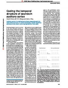
FIG. 2. Response of a simple cell to stationary sinusoidal gratings. A: poststimulus time histograms (1-ms bins) of the response of a V1 simple cell (35/1 s) to sinusoidal gratings presented 100 times at 8 contrasts. The stimuli appear at time 0 and are turned off at 237 ms. Response onset is abrupt, with a latency that decreases as a function of contrast. B: typical responses can be divided into 4 components: the onset latency, the transient period of high firing rate, the elevated tonic firing that follows the transient and persists until the stimulus is turned off, and the off response itself. The procedure for assigning boundaries between response components is described in METHODS. C: firing rate vs. contrast for each response component: full response (▫), transient (E), tonic (‚), and off (ƒ). D: onset latency (䡲) and median first postlatency spike time (●) as a function of contrast.

are generated by discrete mechanisms in the first place, the analysis that follows examines the degree to which each temporal component encodes the contrast of the visual stimulus. The latency (Maunsell and Gibson 1992) is defined as the amount of time between stimulus onset and the beginning of the neural response. In V1 neurons, its duration reflects, at the very least, the time required for a response to be evoked in the photoreceptors and for the neural signal generated in the photoreceptors to pass through the various retinal cell layers and the lateral geniculate nucleus. Latency in V1 neurons decreases as the contrast of the visual stimulus increases (Gawne et al. 1996; Sestokas and Lehmkuhle 1986), a phenomenon that is related to the temporal phase advance of responses to drifting gratings with increasing contrast, in both the retina (Shapley and Victor 1978) and cortex (Albrecht 1995; Dean and Tolhurst 1986). The decrease in latency can be appreciated by scanning down the column of PSTHs in Fig. 2A and observing that the onset of the response becomes progressively earlier as contrast increases. The transient portion of the response is the relatively brief period of intense firing that begins when the visual signal first reaches the neuron. The bulk of the stimulus-related information in neuronal responses has already been transmitted by the end of the transient component (Burac˘as et al. 1998; Heller et al. 1995; Mu¨ller et al. 1999a; Purpura et al. 1993). In the responses of the neuron presented in Fig. 2, the firing rate

increases quickly after the response onset and remains high for 40 –50 ms before declining to a tonic level that is relatively sustained until after the stimulus has been turned off. The decline in firing rate has been thought to reflect a process of short-term adaptation, perhaps involving synaptic depression (Chance et al. 1998; Mu¨ller et al. 1999b). After the tonic response ends, at around 277 ms, a brief off response appears. The off response is much smaller than the transient response, even though the change in contrast is identical (0 to 1 or vice versa). In this simple cell, the relative size of the transient and off responses is largely a function of the spatial phase of the stimulus (not shown). This neuron’s response is similar to that of the “nonlinear simple cell” recorded from cat V1 and depicted in Fig. 5 of Movshon et al. (1978). Of the 50 neurons analyzed here, only 20 had distinct transient and tonic response components that were easily separable by eye and by the boundary-search method (see METHODS). The other neurons had responses that decayed slowly over time or else remained constant until after the grating was removed. Thus conclusions about the contrast-encoding properties of the response latency are based on data from 50 neurons, whereas conclusions about the contrast-encoding properties of the transient, tonic, and off responses are based on data from 20 neurons. Fig. 2, C and D, shows different scalar measures of the contrast responses, plotted against contrast. In Fig. 2C, the firing rate is plotted on a logarithmic scale separately for each temporal response component. The firing rate for the full response (▫) has a dynamic range of about 40 spikes/s, but most of that range is evoked by contrasts of 0.5 and lower. Above this contrast, the firing rate saturates, making it very difficult to distinguish high-contrast stimuli on the basis of firing rate alone. This type of saturation is a common feature of many V1 neurons’ contrast response functions (Ahmed et al. 1997; Albrecht and Hamilton 1982; Maffei and Fiorentini 1973; Tolhurst et al. 1981), and it is prominent in all temporal components of the response. Figure 2D shows the dependence on stimulus contrast of latency (䡲) and median first postlatency spike time (F). The latency is a PSTH-based measure of the earliest time that the response rises above the baseline firing rate. Like the firing rate, both of these response measures change rapidly at low contrast and less rapidly at high contrast, though the degree of saturation is arguably less for latency and first spike time than for firing rate. The decrease in response latency as a function of contrast has been proposed to be a primary way in which visual neurons represent contrast (Bolz et al. 1982; Cleland and Enroth-Cugell 1970; Gawne et al. 1996; Wiener et al. 1999). The relative contribution of each temporal response component to the encoding of contrast is assessed by comparing the information conveyed by subset spike trains that consist only of spikes within a particular response component with average latency information either left intact or removed. In the following sections, full response refers to spikes that occur between the onset latency and a cutoff time 237 ms later. For responses that include a clear transient component (20 of 50 neurons), the full response is extended by the duration of the transient so as to include the off response regardless of its actual size or duration. Latency is determined independently for each contrast but assumes a fixed value for all spike trains recorded at that contrast since it is a measure derived from the

TEMPORAL CODING OF CONTRAST

1043

average response at each contrast. Only contrasts that evoke a clear response onset are considered, so that the full set of contrasts is not necessarily analyzed for each neuron. For each neuron, approximately 100 responses are recorded at each contrast. Latency Latency and firing rate, a priori, are independent response measures. As shown in Fig. 2, both measures covary with contrast. Across all 50 neurons in the sample, stimulus contrast is correlated with both firing rate (median Pearson’s R ⫽ 0.94) and latency (R ⫽ ⫺0.78), and, consequently, the correlation between firing rate and latency is high (R ⫽ ⫺0.86). The degree of correlation is nearly twice as high as what is found in cat retinal ganglion cells for stimuli that vary in spatial position within the receptive field (Levick 1973). To evaluate the separate contributions of firing rate and response latency to the coding of contrast information in V1, it is useful to compare the information transmitted by the full response with the information transmitted by two derived responses. The two derived responses are complementary: one contains only the latency information and the other removes latency information entirely. This means that if the sum of the contrast-related information in the derived responses exceeds the contrast-related information in the full response, the two derived responses can be said to convey redundant information. Alternatively, if the derived responses convey independent information, their information curves are expected to sum to the information curve of the full response. If one of the derived responses conveys more information than the full response, then the additional features in the full response can be said to provide confusing information about contrast (although in that case they may provide information about other stimulus features, such as spatial phase). The first derived response is obtained by subtracting the contrast-specific (but not trial-specific) latency from all spike times recorded at each contrast. This preserves the relative spike times within and across trials at a single contrast but removes the overall latency shift across contrasts. The resulting derived response, which contains the same number of spikes as the original response, as well as the same interspike intervals, is used to evaluate the amount of contrast-related information contained in aspects of the response other than latency. This information could be carried by spike counts and by aspects of temporal pattern other than the time of the first spike (for example, the time of the second spike or the occurrence of “bursts”). The second derived response is obtained by selecting only the first postlatency spike in each trial of the full response. Trials in which no spikes are fired are ignored so that each trial in the derived response has exactly one spike. This removes the confounding effect of differences in spike count since spikefree trials are more likely to occur at lower contrasts. The result is a derived response that is used to evaluate the amount of contrast-related information encoded specifically into the response latency. Figure 3 shows the results of applying the spike metric method to the full and derived responses for two separate neurons. For each cost q, information is expressed as a percentage of the maximum information that would have been obtained from the set of responses if the responses to different

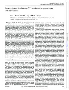
FIG. 3. Information transmitted in the onset latency. Contrast-related information in the full response (▫), in the response with latency removed (E), and in the 1st spike alone (‚). Transmitted information is evaluated by the spikemetric method. A: simple cell from Fig. 2 (35/1 s). B: complex cell (38/2 s). —, empirical fits to the data points (see METHODS). Information values are represented as a percentage of the maximum possible information (log2 N, where N is the number of stimuli), after an estimated bias due to limited sample size is subtracted (see METHODS). Error bars represent 1 SE of the mean and are derived from a bootstrap resampling procedure (see METHODS).

contrasts were perfectly distinguishable. This maximum value, in bits, is log2 N, where N is the number of stimulus conditions. All information estimates (both actual and normalized) are corrected for the small-sample bias by subtracting the information expected from chance clustering. Individual points are fit to an empirical five-parameter curve as described in METHODS. The parameters Hpeak (peak information, possibly equal to the spike-count information H0), ⌰ (temporal coding index), and qcut (temporal precision limit) are extracted from these fits. H0 itself is estimated directly. Figure 3A shows the information curves for the simple cell of Fig. 2. Essentially all of the information in the full response (▫) is encoded in the spike count: H0 is 14% ⫾ 1.4% (SE of the mean derived from 100 bootstrap resamplings), whereas Hpeak is 16% (derived from a fit to the information curve; see METHODS). Although approximately ⌰ ⫽ 8.5% of the contrastrelated information is transmitted by a temporal code, this value is not significantly different from zero. The same is true in the derived response with latency information removed (E; ⌰ ⫽ 2.5%, not significantly different from 0). For this derived response, H0 is by construction equal to H0 of the full response (up to discrepancies in the estimate of information bias; see METHODS) since the number of spikes in each trial of the full and latency-free responses is the same. Remarkably the information in the first spike alone (‚) is as high as the information in the full response (Hpeak ⫽ 15%), which means that the information contained in the time of the first spike is redundant with

1044

D. S. REICH, F. MECHLER, AND J. D. VICTOR

the information contained in the spike count. For the first spike alone, H0 is 0% by construction: all trials in the derived response have exactly one spike so that no information at all is transmitted by the spike count. In addition to showing the amount of contrast-related information transmitted by the first spike compared with the full response, the information curves in Fig. 3A provide insight into the informative temporal precision of spikes in the full and derived responses. As discussed in the APPENDIX, this is a measure of the precision with which spike times can be used to distinguish one stimulus from others, but it is not explicitly related to the reliability of spike times across trials for particular stimuli. One measure of the temporal precision limit is qcut, the value of q at which the fitted information curve Hfit(q) reaches Hpeak/2. For the full response, qcut is 110 s⫺1, giving an informative temporal precision limit of 2,000/qcut ⫽ 18 ms. The temporal precision limit of the response with latency removed is similar (20 ms). These values represent a kind of average over the entire response. However, when the analysis is limited to the first spike alone, the temporal precision limit (assuming there is at least 1 spike in the response) is about twice as fine (10 ms). Figure 3B shows the corresponding information curves for a complex cell. When the latency information is removed from the response of this neuron, less than half of the contrastrelated information remains: Hpeak of the derived response with latency removed is only 44% of Hpeak of the full response. Whereas 62% of the information in the full response is temporally coded, the percentage declines to 15% when the latency information is removed. In this neuron’s response, the first spike alone (‚) transmits far more information than the full response (▫), meaning that later spikes actually impair contrast discrimination. However, the temporal precision limit of the first spike (40 ms) is coarser than the temporal precision limit of the full response (24 ms). Indeed the responses of this neuron highlight the difficulty of interpreting the temporal precision limits derived from the information curves: even though the temporal precision limit is lower for the first spike than for the full response, the first spike transmits more information about contrast than does the full response at any given temporal precision (q). The information curves across all 50 neurons are summarized in Fig. 4, which uses box plots to represent the distributions of each information parameter for the full response and the two derived responses. As expected (Fig. 4A), more contrast-related information is conveyed in the full response (median Hpeak: 8.6%) than in the response with latency removed (3.9%, P ⬍ 0.001, direct comparison with 1,000 paired bootstrap resamplings). However, the first spike alone typically conveys more information than the full response (12%, P ⬍ 0.001). Not surprisingly, then, the sum of the information conveyed by the two derived responses (right-most distribution, 16%) is also larger than the information conveyed by the full response (P ⬍ 0.001), indicating that the contrast-related information in the two derived responses is redundant (Gawne et al. 1996). There are no significant differences between simple (n ⫽ 22) and complex (n ⫽ 28) cells in the median value of Hpeak for either the full response or the two derived responses (P ⬎ 0.05, direct comparison with 1,000 unpaired bootstrap resamplings). Figure 4B shows that contrast is encoded in the full response

FIG. 4. Summary of contrast-related information in the response latency. Distributions are derived from the responses of 50 V1 neurons to stationary sinusoidal grating stimuli. Information parameters are taken from fits to information curves such as the ones shown in Fig. 3. Box plots depict medians (box centers), interquartile ranges (box boundaries), data within 1.5 interquartile range of the medians on both sides (whiskers), and 95% confidence intervals of the medians (notches). ⫹, outliers within the displayed vertical-axis range. Since none of the information parameters can take on values less than 0 and since one of them (⌰) is bounded above by 100%, boxes and whiskers may merge at these extreme values. A: peak information values (Hpeak), expressed as a percent of the maximum possible information. B: estimated percentage of information that is represented by a temporal code (⌰). Because all 1st-spike responses have exactly 1 spike, ⌰ ⫽ 100% by definition. C: informative temporal precision limit, in ms (2,000/qcut). D: informative temporal precision limit of 1st spike alone vs. informative temporal precision limit of full response for each neuron.

primarily through a temporal code: the median temporal coding fraction (⌰) is 61%. Most of this is due to latency variations, and the temporal coding fraction declines to 19% when those variations are removed (P ⬍ 0.001). This confirms that most of the temporally coded information is in the response latency as indexed by the time of the first spike. Again there are no significant differences between simple and complex cells in terms of the median value of ⌰. Figure 4C depicts the distribution of informative temporal precision limits (2,000/qcut) across all neurons. The full responses have a median temporal precision limit of 20 ms,

TEMPORAL CODING OF CONTRAST

1045

significantly finer than the temporal precision limits of the responses with latency removed (median: 24 ms, P ⫽ 0.004) but not significantly different from the temporal precision limits of the first spikes alone (23 ms, P ⫽ 0.06). Figure 4D shows that the temporal precision limits for the full response and the first spike alone are correlated (Spearman’s rank correlation coefficient: 0.51, P ⫽ 0.002, direct comparison with 1,000 paired bootstrap resamplings). There are no significant differences between simple and complex cells with respect to qcut. It is important to reiterate that in the context of the results described here, the informative temporal precision limit gives an estimate of the time differences that are relevant for distinguishing between different contrasts and not of the reliability of a particular spike time within a response across repeated trials (although the two numbers may be correlated). As discussed in the preceding text, the temporal precision limit cannot be considered in isolation from the overall information, which is typically significantly higher for the first spike alone than for the full response. Transient, tonic, and off responses In the responses of 20 of the 50 neurons, transient, tonic, and off components are clearly delineated. To analyze the contrastencoding properties of each temporal component separately, derived responses are constructed that consist only of spikes that occur during one of the response components. From each spike time, the starting time of its associated response component is subtracted. For example, the contrast-specific latency is subtracted from all spike times in the transient response at each contrast. This subtraction means that the comparison of response components is not confounded by differences in the onset times of those components; without the subtraction, responses would be extremely easy to distinguish and information values would be spuriously high. Figure 5A shows the information curves for the simple cell of Figs. 2 and 3A; ▫’s are taken directly from Fig. 3A and represent the contrast-related information conveyed by the full response, whereas E’s represent the transient response, which conveys at most 63% of the peak contrast-related information in the full response and does so with an informative temporal precision limit of 10 ms. The ‚’s represent the tonic response, which conveys 71% as much contrast-related information as the full response with a temporal precision limit of 22 ms. Within the range of decoding schemes parameterized by q, the information contents of the full, transient, and tonic response are most easily evaluated by counting spikes. Finally, the 〫’s represent the off response, which is relatively weak in this neuron at this spatial phase (see Fig. 2A). Not surprisingly, contrast is least well encoded by the off response. Figure 5B shows the information curves for a complex-cell response with very prominent transient and off response components and a tonic response close to the background firing level. For this neuron, the individual response components encode contrast poorly, whereas the full response encodes, at its peak, 41% of the available information about contrast. This information is almost exclusively (⌰ ⫽ 89%) temporally coded and is conveyed in the latency rather than in the temporal structure of the response components (not shown). Across all neurons, the transient and tonic responses and

FIG. 5. Information curves for full response and response components. Full response (▫), transient (E), tonic (‚), and off (〫). Details are as in Fig. 3. A: simple cell (35/1 s), same as Figs. 2 and 3A. B: complex cell (43/11 s).

especially the off response encode substantially less contrastrelated information than the latency or overall spike count, at least for the set of contrasts used here. The median peak information (Hpeak) is significantly lower for each response component than for the full response or the first spike alone (P ⬍ 0.001; distributions not shown). A more appropriate comparison, though, is the one shown in Fig. 6A, where the information-parameter distributions for the full response with latency removed are presented in the first column. This is because the responses derived from the three response components also do not preserve latency variation, as discussed in the preceding text. Hpeak for each of the three components is significantly lower than Hpeak for the full response with latency removed (P ⬍ 0.004). However, when the values of Hpeak are summed across the three response components separately for each neuron, the result is significantly greater than Hpeak of the response with latency removed (medians: 11 vs. 7.1%, respectively, P ⬍ 0.001). This means that the information about contrast conveyed by the three response components is substantially redundant. To the extent that the different response components do encode contrast, the transient is significantly more effective (higher Hpeak) than either the tonic or off component (P ⬍ 0.004). The timing of spikes within the transient and tonic components is not likely to play a primary role in the encoding of contrast (Fig. 6B), although the time at which the transient component begins— equivalent to the latency—is clearly important. Figure 6C shows that spikes are significantly more precise in the transient than in the tonic (P ⫽ 0.02). The fine informative temporal precision estimate for the off responses is most likely an artifact of poor fits to the information estimates, as in Fig. 5A. Finally, among the neurons with responses that

1046

D. S. REICH, F. MECHLER, AND J. D. VICTOR

contrasts may evoke similar responses. The balance of these effects determines whether the transmitted information is larger or smaller when responses to more contrasts are included. Also of interest is whether changing the stimulus set determines the aspects of the responses that are most informative in discriminating among contrasts—in particular, whether the information is primarily encoded in the spike count or spike times and with what precision. Figure 7A shows the dependence of spike count on contrast for a V1 simple cell stimulated with stationary sinusoidal gratings. The response increases over the entire range of contrasts but shows signs of saturating at the highest contrasts. The information curves derived from this neuron’s responses to all

FIG. 6. Summary of contrast-related information in the temporal response components. Distributions are derived from the responses of 20 V1 neurons to stationary sinusoidal gratings. These responses all have distinguishable temporal components (transient, tonic, off). Box-plot details as in Fig. 4.

could be clearly divided into transient, tonic, and off components, there were no reliable differences between simple (n ⫽ 7) and complex cells (n ⫽ 13) in any of the information measures. Information estimates depend strongly on the sampling range and density of stimulus contrast For each neuron tested, the stimulus set consisted of stationary sinusoidal gratings at either an arithmetic series of eight contrasts or a geometric series of six contrasts. The results presented in Figs. 3– 6 are derived from responses to contrasts that evoked a robust change in each neuron’s firing rate in which response-component boundaries could be estimated. Thus the number of contrasts and the particular contrast values analyzed differ from neuron to neuron. To make across-neuron comparisons, information values are normalized by the maximum information available in the stimulus set (i.e., log2 of the number of stimulus categories). However, the calculated information values depend strongly on the particular contrasts that are analyzed and not just on the number of contrasts. Intuitively, this makes good sense: the greater the difference in contrast between two stimuli, the easier to distinguish them and, by extension, to distinguish a neuron’s responses to them. Thus the information transmitted about a pair of stimuli at contrasts 0.125 and 0.25 is expected to be lower than the information transmitted about a pair of stimuli at contrasts 0.125 and 1. As more contrasts are added to the stimulus set, two things happen. First, the maximum information that can be transmitted in response to the entire set increases because the number of stimuli is larger. Second, there is a greater potential for confusing the various contrasts both because there are more of them and because the particular

FIG. 7. Information about contrast depends on the set of stimuli. Responses of a V1 simple cell (43/10 s) to stationary gratings of 4 contrasts (0.125, 0.25, 0.5, and 1). A: firing rate as a function of contrast. Error bars represent 2 standard errors of the mean. B: information curves (bits) and empirical fits for all pairwise combinations of contrasts. Symbols and line type indicate the contrast offset in the pair. Solid lines and open squares: factor of 2. Dashed lines and open circles: factor of 4. Dotted lines and open triangles: factor of 8. Thickness indicates the lower contrast in each pair; thin: 0.125; medium: 0.25; thick: 0.5. Inset: mean value of Hpeak for fixed values of the ratio of higher to lower contrast. C: fits from B, each normalized to its own maximum. In this representation, the information at q ⫽ 0 s⫺1 is the fraction of the total information that is contained in the spike count or firing rate (i.e., 1 ⫺ ⌰/100). This plot reveals that spike count plays a relatively more important role when the contrasts are sparsely sampled (contrast ratio 8); conversely, temporal coding is more important when the contrasts are densely sampled (contrast ratio 2). Inset: mean value of the temporal coding fraction ⌰ for fixed values of the contrast ratio.

TEMPORAL CODING OF CONTRAST

six pairwise combinations of the four contrasts (0.125, 0.25, 0.5, and 1) are shown in Fig. 7B. Here information is given in bits rather than percentages, and the maximum possible transmitted information is 1 bit. Line thickness indicates the lowest contrast in the pair—thin for 0.125, medium for 0.25, and thick for 0.5. Solid lines and squares represent pairs in which the two contrasts differ by a factor of two, dashed lines and circles by a factor of four, and the dotted line and triangle by a factor of eight. Intuitively, one expects that closely spaced contrasts are difficult to distinguish and that information estimates calculated from neuronal responses to pairs of closely spaced contrasts should consequently be low. This intuition accounts for the clustering of information curves by line type (solid, dashed, or dotted), corresponding to different contrast ratios of the stimuli, along the vertical axis in Fig. 7B. The mean value of Hpeak increases with the contrast ratio (ratio of the higher to lower contrast; Fig. 7B, inset). Unexpectedly the fraction of temporally encoded information (⌰/100) decreases with the contrast ratio. This can be seen in Fig. 7C, which plots the fits from Fig. 7B, each normalized to its own maximum. The fraction of information that is encoded in the firing rate (1 ⫺ ⌰/100) is given by the value of each curve at q ⫽ 0 s⫺1; this fraction is greatest when the contrasts of the two stimuli are 0.125 and 1 and least when the contrasts are 0.125 and 0.25. The mean values of ⌰ are plotted as a function of the contrast ratio in Fig. 7C, inset. The neuron of Fig. 7 is typical of the population. This is summarized in Fig. 8, which shows the distributions of the three key response statistics as a function of the contrast ratio. Figure 8A shows that the peak contrast-related information

FIG. 8. Summary of information parameters for responses to pairs of contrasts. Parameters derived from fits to the information curves. Distributions across 50 neurons. Box plots as in Fig. 4. n ⫽ 29 for contrast ratio 8, n ⫽ 63 for contrast ratio 4, and n ⫽ 111 for contrast ratio 2. A: peak information (Hpeak), expressed in bits, greatest for widely separated contrasts (contrast ratio 8). B: temporal coding fraction (⌰), greatest for closely separated contrasts (contrast ratio 2). C: temporal precision limit (2,000/qcut), generally (but not significantly) finest for closely separated contrasts (contrast ratio 2).

1047

Hpeak increases with contrast ratio (P ⬍ 0.0001, KruskalWallis nonparametric ANOVA). On the other hand (Fig. 8B), the relative amount of temporal coding in the response is largest when the contrasts are closely spaced (low contrast ratio) and smallest when the contrasts are far apart (P ⫽ 0.03). The informative temporal precision limits of the spikes that contribute to distinguishing contrasts does not change significantly with contrast ratio (Fig. 8C; P ⫽ 0.15). On the basis of these results, it is proposed that a major role of temporal coding is to enable the visual system to distinguish among stimuli even when there is little change in firing rate. Ultimately, of course, as the difference between the two contrasts is decreased, even the temporally coded information must fall to zero, and the precision of coding is then undefined. DISCUSSION

The results in this paper address two important issues regarding contrast encoding by V1 neurons. First, they provide insight into the detailed temporal structure of responses to stationary sinusoidal gratings and the degree to which information about contrast is encoded in each distinct temporal component. Second, they suggest a hypothesis for the role played by temporal coding in contrast discrimination. Role of different response components The temporal structure of the spike-train response of a visual neuron can be shaped by a number of factors. Most importantly, perhaps, the temporal structure of the response can directly reflect temporal changes in the stimulus. However, information about static features of the stimulus (for the stimuli considered here, contrast, spatial frequency, and orientation) can be multiplexed into the temporal structure of the response (McClurkin et al. 1991; Victor and Purpura 1996). For stimuli that vary rapidly in time, these two sources of temporal modulation in the response are likely to be confounded. The temporal modulation in the stationary stimuli— here, sinusoidal gratings that, after an abrupt onset, are present for 237 ms and then replaced by a uniform field at the same mean luminance—is relatively simple. This makes it possible to study the ways in which stimulus contrast, per se, affects the responses of V1 neurons. Consistent with previous reports, the results indicate that contrast is encoded in both the firing rate and temporal structure of stationary-grating responses. The summary distributions plotted in Figs. 4 and 6 show that, for these stimuli, nearly all the available information about contrast is contained in some combination of firing rate and latency and that at least some portion of that information is encoded redundantly into both aspects of the response. That neurons encode contrast-related information into these two response parameters has been known for some time (Hartline 1938). The present results show that latency, the variation of which can depend precisely on contrast, conveys significantly more contrast-related information than does firing rate in the responses of monkey V1 neurons. In this context, it is important to point out that although the method provides an estimate of the informative temporal precision limits in these responses, it does not prove that such temporal precision is actually used by the brain. To examine this issue directly, experiments would need to be performed in which the perceptual or behavioral

1048

D. S. REICH, F. MECHLER, AND J. D. VICTOR

consequences of manipulating the fine temporal precision of V1 neurons’ responses are examined. From a clinical point of view, the results may be relevant for understanding aspects of visual loss in multiple-sclerosis patients, who tend to have defects in contrast sensitivity that are out of proportion to their loss of visual acuity (Regan et al. 1977). The major pathophysiological effect of chronic demyelination—the primary lesion in multiple sclerosis—is slowing of conduction, which could easily disrupt the finely tuned variations in response latency that are so informative about the contrast of visual stimuli. Thus it is reasonable to speculate that disturbances of the temporal structure of responses may play a critical role in the visual defects seen in demyelinating diseases. It is not immediately clear that cortical neurons can actually obtain an accurate measure of latency, which is a necessary prerequisite for decoding the contrast-related information encoded therein. Determination of latency requires a comparison of response onset to stimulus onset, but the response onset itself is actually the neuronal representation of stimulus onset. A number of solutions to this problem can be proposed. One possibility is that there is an overall population activation in V1 that occurs regardless of the particular visual stimulus. Latency information could then be extracted through a comparison of the response times of particular neurons to the time of this general activation. In all likelihood, the characteristics of the general activation change with stimulus contrast, just as they do for individual neurons. In this case, latency information could potentially be extracted by downstream neurons that measure the distribution (in particular, the variance) of the onset times of responses in an ensemble of nearby neurons. Additionally, if latency is correlated with the degree of synchrony across multiple neurons, postsynaptic “coincidence detectors” would be able to extract the information contained in the latency (Singer 1999). Finally, neurons might be able to measure response latency through a comparison of response onset to the time of occurrence of a preceding saccade, which could be taken as a sign that a new stimulus is present. Each of these solutions can in principle be tested explicitly, although to do so would be a challenge to current experimental techniques. Beyond firing rate and latency, V1 neurons transmit very little information about the contrast of transiently presented visual stimuli. This is consistent with the results of other investigations (Gawne et al. 1996; Wiener et al. 1999) and raises the question of why the responses to stationary gratings contain such prominent temporal variation, reflected in the transient, tonic, and off response components. The present results, together with earlier work, suggest that these response components may primarily transmit information about other stimulus parameters such as orientation, spatial frequency, and spatial phase (Victor and Purpura 1996). For simple cells, in particular, the timing and magnitude of the transient, tonic, and off response components strongly depend on spatial phase (Movshon et al. 1978) and therefore convey a great deal of information about that stimulus attribute (Victor and Purpura 1998). This would follow naturally if different response components reflect the contributions of distinct receptive-field subunits, as has been suggested (Movshon et al. 1978).

Role of temporal coding in the representation of contrast Previous work has explicitly evaluated the role of temporal coding in the representation of stimulus contrast. Victor and Purpura (1996) find that contrast is encoded with higher temporal precision than other stimulus attributes: between 10 and 30 ms. In a related study, Mechler et al. (1998) confirm that contrast can be encoded into the temporal structure of spike train responses but demonstrate that the temporal structure conveys more information when stimuli have transient components than when they do not. Thus temporal coding is prominent in the responses to drifting edges or square wave gratings, just as it is when stimuli appear and disappear abruptly, but less prominent in the responses to drifting sinusoidal gratings. This is perhaps surprising given that the responses to drifting sinusoidal gratings exhibit a prominent phase advance (Albrecht 1995; Dean 1981), which should be reflected in the information measurements. That the phase advance does not give rise to substantial contrast-related information suggests that the variability in the response phase when the stimulus has no transient overwhelms the informative contrast-dependent variation. The present results extend the analysis of contrast representation by demonstrating (Figs. 7 and 8) that temporal coding plays a relatively (but not absolutely) more important role as the contrast ratio decreases. This agrees with findings in the locust olfactory system in which precise spike times make it possible for the animal to discriminate among odorant stimuli that evoke similar firing rates (Stopfer et al. 1997). In V1, temporal coding can better be used to distinguish contrasts that differ by a factor of two than by a factor of eight. This is not to say, of course, that contrasts beyond the saturation point, which give rise to responses with similar firing rates, can be distinguished as efficiently as lower contrasts even when spike timing information is taken into account—in fact, the opposite is true (Fig. 8). Nonetheless the important implication is that temporal coding—in particular, variations in response latency— extends the dynamic range of V1 responses with respect to contrast representation beyond what would be available from differences in firing rate alone. APPENDIX

In this Appendix, simulations are presented to test the suitability of the metric-space method for calculating information when there are only one or two spikes per trial. This is akin to the situation, described in RESULTS, in which derived spike trains that contain only the first spike in a response are evaluated. More general simulations that test the metric-space method under a variety of conditions are presented in Victor and Purpura (1997). The simulated response sets analyzed in this appendix each consists of two stimulus conditions. Within each condition, the spike times are drawn from either one or two Gaussian distributions, one spike per distribution. The means and SDs of the distributions and the overall offset of the distribution means between conditions are the parameters that are varied in the simulations. For each condition, a fixed number of trials are simulated, each of which contains the same number of spikes (either 1 or 2). The simulated spike trains are subjected to the metric-space analysis, and the results are compared with the results of an analysis in which a simulated response is assigned to the stimulus category that has the highest likelihood of giving rise to spikes at the observed times (Cover and Thomas 1991). The latter analysis is performed on 10,000 simulated spike trains from the same underlying

TEMPORAL CODING OF CONTRAST

FIG. A1. Metric-space results for simulated data. Test of the suitability of the metric-space method for estimating information and temporal precision when the number of spikes per trial is low. A: bias-corrected information as a function of the cost q (left) and the number of simulated trials (right). Left: different curves represent different numbers of simulated trials: 16 (open squares), 64 (open circles), 128 (open triangles), and 1,024 (inverted open triangles). Right: different curves represent different values of q: 1 (open squares), 8 (open circles), 64 (open triangles), and 512 (inverted open triangles) s⫺1. B–D: peak information (Hpeak) and temporal precision limits (2,000/ qcut) derived from fits to the information curves. Left: solid lines show expected information values from a likelihood-ratio analysis. Right: solid lines show expected temporal precisions for different mean separations (slanted lines) and standard deviations (horizontal lines) of the Gaussian distributions that are used to generate spike times. Symbols correspond to different ratios of mean separation to standard deviation: 1 (open squares), 4 (open circles), and 16 (open triangles). B: 1 spike/trial. C: 2 spikes/trial; spike-time distributions within a trial have a mean separation of 32 ms. D: 2 spikes/trial (same data as in C) but only the 1st spike in each trial is analyzed.

distributions—100 times more trials than are available from real data. In cases when there is only one spike per trial, it is easy to calculate the information explicitly from the probability distributions; the information values derived from the likelihood-ratio analysis match the true information values very well. Figure A1A shows the effects of varying the cost parameter q and the number of simulated trials on the estimated information. In this example, there is only one spike per trial. The separation between distribution means across conditions is 16 ms, and the distributions have a standard deviation of 8 ms (so that there is considerable overlap that can lead to ambiguity in assigning responses to the appropriate stimuli). Figure A1A, left, shows the bias-corrected information values as a function of q for four different sets of simulated responses, each of which contains a different number of trials: 16 (open squares), 64 (open circles), 128 (open triangles), and 1,024

1049

(inverted open triangles). The — shows the actual information (0.37 bits) calculated analytically. For low values of q, the calculated information is close to the actual information at least when there are a sufficient number of trials. For higher values of q, the information declines to zero, which is expected because spike times measured with extremely high temporal precision do not provide information about the stimulus (Victor and Purpura 1997). Figure A1A, right, shows estimated information plotted against the number of trials simulated for four different values of q: 1 (open squares), 8 (open circles), 64 (open triangles), and 512 (open inverted triangles) s⫺1. When the number of trials is on the order of 100 —the number of trials at each contrast in the real data described in this paper—the calculated information approaches the actual information when q is sufficiently low. The similarity of the curves for different values of q indicates that the accuracy of the bias-correction method does not depend strongly on q, even though it can do so in principle (Victor and Purpura 1997). Figure A1, B–D, shows the results of varying the mean separation and standard deviation of the Gaussian distributions. The left panels plot Hpeak (the maximum calculated information), and the right panels plot 2,000/qcut (the measure of informative temporal precision used in this paper). Both parameters are derived from fits of the information curves (see METHODS). Different symbols correspond to different ratios of mean separation to standard deviation: 1 (open squares), 4 (open circles), and 16 (open triangles). For each condition, 100 simulated spike trains are created. Solid lines in the left panels correspond to likelihood-ratio information measures. Slanted lines in the right panels correspond to estimated temporal-precision limits, which are related to the mean separation between distributions used in the simulations. They are independent of the standard deviations (horizontal lines) because the informative temporal precision corresponds to reliable variations in spike timing across stimulus conditions that can provide information about the stimulus rather than jitter of particular spike times across trials within a condition. The estimated temporal precisions for the stimuli used in these simulations are expected to fall at the intersections of the horizontal and slanted lines. Figure A1B shows the case of one spike per trial; a subset of these data is plotted, in more detail, in Fig. A1A. Figure A1C shows the case of two spikes per trial, where the individual spike-time distributions within each trial are separated by 32 ms. Figure A1D shows the results of extracting the first spike from each of the trials in Fig. A1C and performing the metric-space analysis; this corresponds to extracting the first postlatency spike at each contrast in real data. The results indicate that the estimated information values for 100 trials are generally very close to the expectation, regardless of the mean-separationto-standard-deviation ratio, in all three simulations (left). Moreover, the calculated temporal precision limits fall near the intersections of the horizontal and slanted lines in the right panels, indicating that the temporal precision is recovered relatively accurately by the metricspace method. Together with the results of Victor and Purpura (1997), the simulations reveal that the metric-space method, as used here, can accurately estimate information and informative temporal precision limits from spike data. We thank B. Knight and K. Purpura for many helpful comments. This work was supported by National Institutes of Health Grants GM-07739 and EY-07138 (D. S. Reich) and EY-9314 (J. D. Victor). REFERENCES AHMED B, ALLISON JD, DOUGLAS RJ, AND MARTIN KA. An intracellular study of the contrast-dependence of neuronal activity in cat visual cortex. Cereb Cortex 7: 559 –570, 1997. ALBRECHT DG. Visual cortex neurons in monkey and cat: effect of contrast on the spatial and temporal phase transfer functions. Vis Neurosci 12: 1191– 1210, 1995. ALBRECHT DG AND HAMILTON DB. Striate cortex of monkey and cat: contrast response function. J Neurophysiol 48: 217–237, 1982.

1050

D. S. REICH, F. MECHLER, AND J. D. VICTOR

BOLZ J, ROSNER G, AND WASSLE H. Response latency of brisk-sustained (X) and brisk-transient (Y) cells in the cat retina. J Physiol (Lond) 328: 171–190, 1982. BONDS AB. Temporal dynamics of contrast gain in single cells of the cat striate cortex. Vis Neurosci 6: 239 –255, 1991. BURAC˘ AS GT, ZADOR AM, DEWEESE MR, AND ALBRIGHT TD. Efficient discrimination of temporal patterns by motion-sensitive neurons in primate visual cortex. Neuron 20: 959 –969, 1998. CHANCE FS, NELSON SB, AND ABBOTT LF. Synaptic depression and the temporal response characteristics of V1 cells. J Neurosci 18: 4785– 4799, 1998. CLELAND BG AND ENROTH-CUGELL C. Quantitative aspects of gain and latency in the cat retina. J Physiol (Lond) 206: 73–91, 1970. COVER TM AND THOMAS JA. Elements of Information Theory. New York: Wiley, 1991. DEAN AF. The relationship between response amplitude and contrast for cat striate cortical neurones. J Physiol (Lond) 318: 413– 427, 1981. DEAN AF AND TOLHURST DJ. Factors influencing the temporal phase of response to bar and grating stimuli for simple cells in the cat striate cortex. Exp Brain Res 62: 143–151, 1986. DEANGELIS GC, GHOSE GM, OHZAWA I, AND FREEMAN RD. Functional microorganization of primary visual cortex: receptive field analysis of nearby neurons. J Neurosci 19: 4046 – 4064, 1999. EFRON B AND TIBSHIRANI RJ. An Introduction to the Bootstrap. Boca Raton, FL: Chapman and Hall/CRC, 1998. GAWNE TJ, KJAER TW, AND RICHMOND BJ. Latency: another potential code for feature binding in striate cortex. J Neurophysiol 76: 1356 –1360, 1996. HARTLINE HK. The response of single optic nerve fibers of the vertebrate eye to illumination of the retina. Am J Physiol 121: 400 – 415, 1938. HEEGER DJ. Normalization of cell responses in cat striate cortex. Vis Neurosci 9: 181–197, 1992. HELLER J, HERTZ JA, KJAER TW, AND RICHMOND BJ. Information flow and temporal coding in primate pattern vision. J Comput Neurosci 2: 175–193, 1995. IKEDA H AND WRIGHT MJ. Spatial and temporal properties of “sustained” and “transient” neurones in area 17 of the cat’s visual cortex. Exp Brain Res 22: 363–383, 1975. LENNIE P. The physiological basis of variations in visual latency. Vision Res 21: 815– 824, 1981. LEVICK WR. Variation in the response latency of cat retinal ganglion cells. Vision Res 13: 837– 853, 1973. MAFFEI L AND FIORENTINI A. The visual cortex as a spatial frequency analyser. Vision Res 13: 1255–1267, 1973. MAUNSELL JH AND GIBSON JR. Visual response latencies in striate cortex of the macaque monkey. J Neurophysiol 68: 1332–1344, 1992. MCCLURKIN JW, OPTICAN LM, RICHMOND BJ, AND GAWNE TJ. Concurrent processing and complexity of temporally encoded neuronal messages in visual perception. Science 253: 675– 677, 1991. MECHLER F, VICTOR JD, PURPURA KP, AND SHAPLEY R. Robust temporal coding of contrast by V1 neurons for transient but not for steady-state stimuli. J Neurosci 18: 6583– 6598, 1998. MILLER GA. Note on the bias on information estimates. Inform Theor Psychol Probl Methods II-B: 95–100, 1955.

MOVSHON JA, THOMPSON ID, AND TOLHURST DJ. Spatial summation in the receptive fields of simple cells in the cat’s striate cortex. J Physiol (Lond) 283: 53–77, 1978. ¨ MULLER JR, MEHTA AB, KRAUSKOPH J, AND LENNIE P. Why onset transients in responses of V1 neurons provide the most reliable information. Soc Neurosci Abstr 25: 1549, 1999a. ¨ MULLER JR, METHA AB, KRAUSKOPF J, AND LENNIE P. Rapid adaptation in visual cortex to the structure of images. Science 285: 1405–1408, 1999b. OHZAWA I, SCLAR G, AND FREEMAN RD. Contrast gain control in the cat visual cortex. Nature 298: 266 –268, 1982. PURPURA K, CHEE-ORTS MN, AND OPTICAN LM. Temporal encoding of texture properties in visual cortex of awake monkey. Soc Neurosci Abstr 19: 315, 1993. REGAN D, SILVER R, AND MURRAY TJ. Visual acuity and contrast sensitivity in multiple sclerosis– hidden visual loss: an auxiliary diagnostic test. Brain 100: 563–579, 1977. REICH DS, MECHLER F, PURPURA KP, KNIGHT BW, AND VICTOR JD. Multiple timescales are involved in coding of contrast in V1. Soc Neurosci Abstr 24: 1257, 1998. REICH DS, MECHLER F, PURPURA KP, AND VICTOR JD. Interspike intervals, receptive fields, and information encoding in primary visual cortex. J Neurosci 20: 1964 –1974, 2000. SCLAR G. Expression of “retinal” contrast gain control by neurons of the cat’s lateral geniculate nucleus. Exp Brain Res 66: 589 –596, 1987. SCLAR G, LENNIE P, AND DEPRIEST DD. Contrast adaptation in striate cortex of macaque. Vision Res 29: 747–755, 1989. SESTOKAS AK AND LEHMKUHLE S. Visual response latency of X- and Y-cells in the dorsal lateral geniculate nucleus of the cat. Vision Res 26: 1041–1054, 1986. SHAPLEY RM AND VICTOR JD. The effect of contrast on the transfer properties of cat retinal ganglion cells. J Physiol (Lond) 285: 275–298, 1978. SINGER W. Time as coding space? Curr Opin Neurobiol 9: 189 –194, 1999. SKOTTUN BC, DE VALOIS RL, GROSOF DH, MOVSHON JA, ALBRECHT DG, AND BONDS AB. Classifying simple and complex cells on the basis of response modulation. Vision Res 31: 1079 –1086, 1991. STOPFER M, BHAGAVAN S, SMITH BH, AND LAURENT G. Impaired odour discrimination on desynchronization of odour-encoding neural assemblies. Nature 390: 70 –74, 1997. TOLHURST DJ, MOVSHON JA, AND THOMPSON ID. The dependence of response amplitude and variance of cat visual cortical neurones on stimulus contrast. Exp Brain Res 41: 414 – 419, 1981. TREVES A AND PANZERI S. The upward bias in measures of information derived from limited data samples. Neural Comput 7: 399 – 407, 1995. VICTOR JD AND PURPURA KP. Nature and precision of temporal coding in visual cortex: a metric-space analysis. J Neurophysiol 76: 1310 –1326, 1996. VICTOR JD AND PURPURA KP. Metric-space analysis of spike trains: theory, algorithms and application. Network 8: 127–164, 1997. VICTOR JD AND PURPURA KP. Spatial phase and the temporal structure of the response to gratings in V1. J Neurophysiol 80: 554 –571, 1998. WIENER MC, ORAM MW, AND RICHMOND BJ. Latency is a better temporal code than principal components. Soc Neurosci Abstr 25: 1549, 1999.