Texture Particles: Interactive Visualization of Volumetric Vector Fields Stefan Guthe, Stefan Gumhold, Wolfgang Straßer WSI/GRIS University of T¨ubingen
[email protected]
ABSTRACT This paper introduces a new approach to the visualization of volumetric vector fields with an adaptive distribution of animated particles that show properties of the underlying steady flow. The shape of the particles illustrates the direction of the vector field in a natural way. The particles are transported along streamlines and their velocity reflects the local magnitude of the vector field. Further physical quantities of the underlying flow can be mapped to the emissive color, the transparency and the length of the particles. A major effort has been made to achieve interactive frame rates for the animation of a large number of particles while minimizing the error of the computed streamlines. There are three main advantages of the new method. Firstly, the animation of the particles diminishes the inherent occlusion problem of volumetric vector field visualization, as the human eye can trace an animated particle even if it is highly occluded. The second advantage is the variable resolution of the visualization method. More particles are distributed in regions of interest. We present a method to automatically adjust the resolution to features of the vector field. Finally, our method is scalable to the computational and rasterization power of the visualization system by simply adjusting the number of visualized particles. Keywords: flow visualization, vector field visualization, flow animation, steady flow, splatting.
1 Introduction The number of new applications in the area of Computational Fluid Dynamics is constantly increasing while at the same time the dataset complexity is also increased. The need for visualization methods is not exhausted yet. Although the problem has been studied thoroughly in two dimensions for volumetric vector fields new challenges are arising. The major problem in three dimensions is the occlusion problem. The human visual system works on the basis of 2d images. One eye produces 2d images while two eyes produce 2d images with additional depth information. All visualization methods have to project their interpretation of the vector field into a two dimensional image. The simplest method is to slice the vector field and use a hedgehog method. But here the global structure of the vector field may be lost. If the complete volume of the dataset is projected into two dimensions because of occlusion only the surface of the dataset can be seen. Three possible workarounds are a transparent visualization, a sparse sampling of the vector field
or feature extraction. Feature extraction is very difficult for three dimensional vector fields because there is a much larger variety of features and it is not clear how to illustrate them intuitively. The use of transparency and sparse sampling only diminish the occlusion problem slightly. Even for a scalar field a transparent rendering gives a depth impression only, when the dataset is rotated interactively. As a volumetric vector field contains much more information than a scalar field, a simple transparent visualization will fail. In the case of a sparse sampling of volumetric vector fields it is very difficult to get an idea of the visual order of the samples without additional cues. Our new visualization method combines the use of transparency with an adaptive sampling. We use transparent arrow shaped or comet like particles as samples, which intuitively show the direction of the vector field. It is also possible to use any of the icons proposed by Walsum et al. [11]. The perception of the depth ordering is improved by adding a halo around each par-
ticle and by the high occlusion of the particles. The changing of the occlusion by animating particles gives further cues about the depth ordering. And at the same time the human eye is able to track even highly occluded particles deep inside the vector field with the help of the motion coherence. In this way the sampling density can be increased with a deeper insight into the interior of the vector field. The length and the speed of the particles in the animation reproduce the magnitude of the vector field in a natural way. A second major advantage of the use of particles is that the visualization resolution can locally be adapted to the resolution of a vector field with highly varying sampling resolution. We also show how to accentuate vector field features by increasing the sampling resolution in their surrounding. Again the animation of the particles improves the understanding of the different kinds of features very intuitively. Thus we can visualize vector field features without the need of actually extracting and visualizing them. A further important advantage of our method is the low pre-computation time and the interactive frame rates, which can be guaranteed also on low-end machines by reducing the number of visualized particles. This does not imply a reduction of the sampling resolution of the vector field as the particles can be focused on any arbitrary region. 1.1 Related Work Z¨ockle et al. [14] introduce an interactive algorithm for visualization of flow data using a sparse representation of the vector field. They visualize a large number of very fine illuminated streamlines, which are preferably initiated near features of the vector field. It is difficult to visualize further physical quantities and the depth impression is only good for a very sparse sampling of the vector field. Wijk [12] extends the streamline approach to stream surfaces by the use of parametric surfaces. The extraction of stream surfaces gives a good overview over the global properties of the vector field, but views at several depths are not possible at the same time, since the stream surfaces are opaque. Raycasting several of these stream surfaces as proposed by Fr¨uhauf [5] permits the perception of several stream surfaces in different depths, but the low sampling resolutions orthogonal to the stream surfaces is disturbing. It is also very tricky to locate critical points of the flow without visualizing them separately, but the main drawback is that the difference of the vector length between two stream surfaces can not be seen.
For the 2d case Line Integral Convolution (LIC, see Cabral and Leedom [1]) is one of the best ways to visualize a vector field in two dimensions because it generates a dense representation of the vector field. Although it does not explicitly extract streamlines the resulting pictures are very similar to the ones generated with streamlines. To combine a good global overview and the visualization of critical points, Interrante and Grosch [6] generalize the LIC to volumetric vector fields, while H. W. Shen et al. [10] use threeand two-dimensional LIC to visualize local and global properties of the vector field. The density of the LIC representation makes it almost perfect for two dimensional vector fields but rather unsuitable for volumetric vector fields because of the extreme amount of occlusion. Simple particle tracing uses only points as particles and therefore represents the vector field direction only through the particle animation. The larger the particle and the more complex it is, the fewer particles can be visualized without confusing the observer. Visualizing flow data with a probe as proposed by Leeuw and Wijk [4] gives a good impression of the local surrounding of the particle but cannot provide a global overview of the whole vector field or the global topology. Crawfis and Max [2] took a different splatting approach to render the scalar and vector valued fields by encoding the vectors with particles that reside on the texture used by the splatting algorithm. The particles in their method have the shape of little blobs that fade along the direction of the vector field.
1.2 Paper Overview The visualization of volumetric vector fields using particles leads to several tasks. Starting with a vector field, we present a way to visualize local properties of the field using a single particle. After being able to set up a particle, we introduce an accurate method to move a particle along a streamline while maintaining a certain distribution within the vector field. After this, the animated particles are displayed using our textured based approach. In section 2 we describe how to find a vector for any location in space using tri-linear interpolation. Section 3 describes how to animate particles along streamlines and how to distribute them within the vector field. In section 4 we explain how the particles are rendered and which problems arise that way. The visualization pipeline is briefly explained in section 5. Finally, we give some results on the performance of our method in section 6.
2 Fast Data Access In order to visualize a vector field using particles that represent properties of the underlying field, we need to know the vector and the additional parameters for any location in space and therefore the relative position within the dataset. Due to the non-regularity of the underlying grid of real world vector fields, we have to solve two main problems. We need a fast interpolation within every type of primitive in the dataset and a fast way to find the corresponding primitive for any given location in space.
The interpolation that has been used during the creation of the dataset can not be reconstructed in general. Therefore we need to define a local steady interpolation within each cell of the grid. There are mainly four different primitives used for a cell within a dataset representing a vector field, the tetrahedron, the pyramid, the triangular prism and the hexahedron cell. While the interpolation within a tetrahedron is rather straight forward, the other three schemes are not that simple. The easiest way to define an interpolation is to split the cells into tetrahedra and interpolate within each tetrahedron using a matrix. Beside the huge amount of matrices, the resulting grid and therefore the interpolation are not unique. To define an interpolation within a primitive consisting of n vertices requires the inversion of a n × n matrix. Although inverting these matrices can be carried out quiet fast this leads to a huge overhead for storing the resulting matrices. Assuming that the surface of each primitive is nearly plane, which can safely be assumed for most of the datasets used in the area of Computational Fluid Dynamics, we can use a different, more effective approach. With vn as the vector at the point pn and the distances dn to describe the position within the primitive, leads to the following interpolation for a tetrahedron (see figure 1a for the naming of the distances): d0 v0 + d1 v1 + d2 v2 + d3 v3 d0 + d1 + d2 + d3
(1)
Using a bi-linear interpolation on the quadrangle of the pyramid and a linear interpolation between the bottom and the top of the pyramid, using the distances seen in figure 1b, results in the following interpolation: a0 =
d0 v0 + d1 v1 d0 + d1
b)
c)
d) Figure 1: Relative position of point l within each primitive.
2.1 Interpolation
v=
a)
(2)
a1 = b = v =
d0 v2 + d1 v3 d0 + d1 d2 a0 + d3 a1 d2 + d3 d4 v4 + (d0 + d1 + d2 + d3 )b d0 + d1 + d2 + d3 + d4
The interpolation for the triangular prism can be split into a bi-linear interpolation on the two opposite triangles and a linear interpolation between them. Using the distances seen in figure 1c results in the following interpolation: a0 = a1 = v =
d0 v0 + d1 v2 + d2 v4 d0 + d1 + d2 d0 v1 + d1 v3 + d2 v5 d0 + d1 + d2 d3 a0 + d4 a1 d3 + d4
(3)
Finally the interpolation for the hexahedron is a simple tri-linear interpolation using the distances seen in figure 1d. a0 = a1 = a2 = a3 = b0 = b1 = v =
d0 v0 + d1 v1 d0 + d1 d0 v2 + d1 v3 d0 + d1 d0 v4 + d1 v5 d0 + d1 d0 v6 + d1 v7 d0 + d1 d2 a0 + d3 a1 d2 + d3 d2 a2 + d3 a3 d2 + d3 d4 b0 + d5 b1 d4 + d5
(4)
Although these calculations can be carried out very fast, the results are not linear within the cell, because the sum of the distances is not constant. On the other hand the interpolation used during construction may also not have been linear. The later algorithm needs fewer space and time than splitting the primitives into tetrahedra and by far less precomputational time than the one using inverted matrices.
a)
b) Figure 2: Building of bsp-tree with a single plane or single references to every cell.
2.2 Finding Cells We are now able to calculate an interpolation within a cell, but we still need a way to find the cell containing the given point. Although this might not seem necessary because animated particles could find the new cell using the neighborhood information of the grid, we still need these cells for inserting new particles. De Berg et al. [3] stated that the problem of point inclusion in 3D can not be solved in general in log(n) time, where n is the number of primitives to be checked and that no optimal algorithm is known. The simplest but inefficient way to find the corresponding cell would be to check every cell whether it contains the point or not. Although this is still quite fast for about 100 cells if a bounding box check is done first, large datasets can not be visualized this way. To reduce the number of cells to be tested for large datasets a bsp-tree can be used. Although this would theoretically result in a search time of log(n), there might always be cells intersecting the split plane of the tree. Therefore the intersecting cells have to be stored in both parts of the bsp-tree (as seen in figure 2a). To reduce the number of cells to be tested effectively we have to construct a bsp-tree by splitting the dataset into two more or less evenly sized parts while producing as few duplicate cells as possible. This would require a balanced bsp-tree as described by de Berg et al. [3] that can not be constructed in general without limiting us to curvilinear grids. To reduce the number of possible planes to split at, we only allow splits in the direction of the x, y and z-axis, resulting in a rectangular bsp-tree and a faster search for the leaf that contains our current location. To construct a balanced bsp-tree while using the most easy to handle planes (those along the three axis), we use a three dimensional kd-tree (see de Berg et al. [3]). We split the dataset using all three possible planes and choose the one producing the least overhead. This results in a nearly balanced bsptree while trying to minimize the overhead. However splitting the dataset until it can’t be split any further, i.e. no edge of any bounding box is inside our node of the bsp-tree, would result in a huge overhead as a single cell may be stored in a
large number of leafs. To handle more complex datasets, we need an approach that does not need any additional memory to store multiple references to each cell and therefore enables us to split the dataset until only a single cell is contained in every leaf of the bsptree. As seen in figure 2b, we split the dataset rather than the space at the current plane. The resulting planes of the bounding box are stored in the bsp-tree rather than the one used for splitting the dataset, because both parts of the tree have to be tested if our current location is between these two planes. Therefore we can not guarantee that only one leaf is needed to find the corresponding cell. In the worst case it might even be possible that a region of the dataset is present in every leaf of the tree and therefore every cell has to be tested. This approach reduced the number of tests to an average of 1.58 using the Oxygen Post dataset (see figure 7) and is therefore faster than using neighborhood information. The overhead of this algorithm, i.e. the space contained in more than one leaf, can be seen in section 6 table 1. 3 Animated Particles Being able to visualize a single particle leaves three problems for animating a large amount of them. We need a scheme to distribute any number of particles within the dataset. We need a fast way to move a particle along the vector field, i.e. a streamline has to be computed. In addition we also have to track them during their movement to remove particles at undesired locations and insert new ones. 3.1 Distribution of Particles We need a distribution of particles to achieve a high sampling resolution in interesting regions of the vector field and a lower one in less interesting ones. There are several characteristics that can be of interest. First of all the density or other physical attributes attached to a flow field might be correlated to the importance of a region, including the magnitude of the vector field. The cur-
vature and the square norm of the divergence as defined by Leeuw and van Wijk [4], normalized with the local magnitude may also correlate to the importance. Thus we come up with the following definition of a weight function: ω(x) = ωconst + ω1 (x) + . . . + ωn (x) +(5) ω(x)grad + ω(x)div + ω(x)curv While ωconst is the amount of homogeneously distributed particles, the weights ωi (x) allow consideration of the different physical quantities of the vector field to influence the particle distribution. Finally, ω(x)grad , ω(x)div and ω(x)curv incorporate the local gradient, divergence and curvature of the vector field. The function ω(x) can also be extended to handle the local shear and rotation of the vector field or any additional function, such as the distance to the closest critical point. Now we can define a weight for any position within the vector field but we still need a way to distribute the particles according to these weights. In order to distribute newly created particles, we introduce the distribution octree. Every leaf gets its weight assigned by sampling the weighting function. Each node in this octree stores the weight of all its children. In each knot the number of actually contained particles is stored and initialized to zero at the beginning. Each time a new particle is created, the distribution octree is traversed from top to bottom, the cell with the most missing particles is located and the particle is placed randomly inside this cell. The distribution octree is dynamically coarsened and refined during the insertion and the removal of particles. A leaf, that should contain more then eight particles, is split while a node that contains children of which each should hold less than one particle is combined to a single leaf. The distribution octree after insertion of all particles for the Blunt Fin dataset is shown in figure 3. To optimize the memory allocation we store the removed octree cells during coarsening in a linked list (as proposed in [7]) in order to speed up cell creation during refinement. 3.2 Movement The fastest way to compute streamlines is a single step Euler integrator. Although it is suitable for a quick preview, it can not be used for most of the present vector fields due to its large error. The best choice between performance and error of the computed streamlines is a fourth order Runge-Kutta integrator with adaptive step width as described by Press et al. [9].
Figure 3: Distribution octree for 10000 particles with a maximum of 16 particles per leaf (Blunt Fin dataset).
Although the integration is very fast for small datasets, there is a huge overhead for larger ones due to the randomness of the memory access produced by particles at different locations. To localize most of the memory access the distribution octree can be used. The algorithm starts with one leaf and moves every particle in it before moving to the next one. Therefore we can test the cell that contained the previous location first. 3.3 Updating After the particles have been moved along the vector field their distribution changed and regions of low interest may contain more particles than they are supposed to, while regions of high interest may contain too few. For removing misplaced particles and inserting them at a different location we need to know the current distribution of particles within the distribution octree. So we need to keep the number of particles per cell up to date while they are moving. But just replacing particles at undesired locations leads to a heavy flickering that prevents the user to see any properties of the vector field if the particles are animated. To reduce the amount of particles being removed during each step of the animation, every particle gets an age property attached. This age allows a particle to stay in an overcrowded region for some time before it will be removed, thus ensuring that a particle is visible for at least a defined number of frames, allowing the user to trace it’s motion. Particles that sometimes visit overcrowded regions but mainly move along undercrowded ones need not be removed. To keep these particles, we reduce their age while they are in undercrowded regions and only increase the age of additional particles in overcrowded ones. This also leads to a minimum number of particles in each region even if there are constantly too many particles present. This can be implemented by us-
ticle are adjusted by scaling the rendering rectangle accordingly. Finally the rotation around the z-axis is performed by rotating the rendering rectangle around the z-axis.
Figure 4: Part of two different textures used for rendering particles.
ing the list of particles in each leaf used for optimization in the last section. Although this reduces the flickering as much as possible while keeping the correct distribution of particles, there is still another way to diminish it further. The flickering is produced by particles that are removed from one location and are created at another at the same time. So we have to fade them out after they reach their maximum age and fade them in again after creation instead of ”teleporting” them to their new location. As a result of this technique there is nearly no visible flickering left.
4 Display Visualizing a huge amount of extended, transparent particles would be very slow if they were rendered using their correct geometry. On the other hand, image based rendering would also be slow or need a huge amount of texture memory, if we desire the perspective to be correct. This tradeoff between speed and accuracy leads to a simple texture based approach. 4.1 Rendering We need a fast and simple texture based approach to render each particle using only one rectangle and therefore only one texture per particle. Moving this rectangle to the particle’s location fixes three degrees of freedom. There are five degrees of freedom left: three for the orientation of the particle and two for its length and diameter. The orientation can be specified by three rotations along the three coordinate axes. Let us assume the particle is aligned with the x-axis. The first rotation around the x-axis can be avoided by choosing rotationally symmetric particles. The rotation around the y-axis is performed by selecting the correct pre-rendered arrows or comet like shapes from one of the textures shown in figure 4, which sample the rotation around the y-axis densely. Next the length and diameter of the par-
Being able to render a single particle we need a simple approach to render all of them. An additional alpha buffer would probably slow down the rendering so we have to sort the particles and render them from back to front using simple alpha blending. Neglecting the particle’s geometry, we only have to sort them according to distance from the viewer to their center of gravity in world coordinates. Because the number of particles is moderate for a sorting problem, we can use the hashing algorithm proposed by Mueller et al. [8]. To use this algorithm effectively we subdivide the interval of all currently used distances equidistantly into twice the number of particles and use these subintervals as hash entries. Each of these entries contains a linked list storing the particles sorted by their distance to the viewer within the corresponding interval. Using this simple approach leads to a linear sorting time in the average case. Although this simple texture based rendering is very fast, it has some major drawbacks. The distance between the viewer and the particle is ignored, resulting in a wrong perspective for most of the particles. The particle is rotated after being scaled while the texture is rotated first and therefore the scaling changes the rotation angle. The distortion caused by the distance to the viewer can not be corrected without using more than one texture per particle or a set of textures as seen in figure 4 for different perspectives. The distortion caused by scaling of the particle can partly be removed if we take a closer look at the resulting transformations. The length of the particle is scaled √ by s while it’s diameter is scaled by s0 = 1/ s to keep the same volume. After this the particle is rotated by α. On the other hand the texture with the rotational angle of β is chosen and scaled by xs, ys and zs to simulate the original transformation. This leads to the following relations. (scosα, 0, s0 sinα) = (xscosβ, 0, xssinβ) (0, s0 , 0) = (0, ys, 0) (−ssinα, 0, s0 cosα) = (−zssinβ, 0, zscosβ) (6) As the scaling to zs along the z-axis is lost during the projection to the final image, the following values for the texture correspond to any given particle. µ
tanα β = atan √ s3 cosα xs = s cosβ
(7)
ys =
1 √ s
For higher rendering performance we only use one texture and render the particle from 512 different angles of y-rotation representing 180 degrees. This is a good compromise between quality of the particles and sampling density of the rotation along the y-direction. By now, we assumed that the viewing vector is along the z-axis and the view up vector is the y-axis. To calculate the coordinates of the textured rectangle using any arbitrary camera direction vdir and position vpos of a particle at the position ppos with the direction pdir we define the relative position and direction of the particle; vdir and pdir are normalized vectors. rpos = ppos − vpos vdir × pdir rup = |vdir × pdir| vdir × rup rfwd = − |vdir × rup| α = asin(rpos · pdir)
(8)
After computing xs, ys and β using equation 7 the textured rectangle p0...3 can be drawn using texture n out of 512 textures as seen in figure 4. n p0 p1 p2 p3
= = = = =
255.5 + 511β/pi (9) ppos − xs/2 · rfwd − ys/2 · rup ppos + xs/2 · rfwd − ys/2 · rup ppos − xs/2 · rfwd + ys/2 · rup ppos + xs/2 · rfwd + ys/2 · rup
4.2 Textures Our technique strongly depends on a good visualization of the particles. The main demands on the particle visualization are that each particle shows the direction and vector length of the visualized flow at the particle location and that the particles are transparent. The direction and vector length can be nicely represented with an arrow or a comet like shape. In order to achieve a high rendering quality of the particles, they where prerendered with a ray-tracer using high over sampling. The pre-rendered particles contain luminance and absorption values, such that further attributes can be visualized through the hue and saturation values of each particle. To allow deep insight into the vector field while maintaining a depth perception for each particle requires the particles to be transparent
Figure 5: top left to bottom right: Non transparent, constant transparency, varying transparency, varying transparency with added halo.
and occluding at the same time. The top left image in figure 5 shows non transparent particles resulting in a good depth perception but only few insight into the vector field. Using a constant transparency of 50% as seen in the top right image results in better insight into the vector field, but the depth perception is nearly lost. Varying the transparency with the thickness of the particle for each pixel, as seen in the bottom left image, does not improve the depth perception significantly. To improve the result any further we need to apply a halo like the one used by Westover [6] that does not reduce the overall transparency of each particle and therefore the insight into the vector field but improves the depth perception. It is also improved by a simple lighting algorithm that scales the brightness of each particle according to its distance to the viewer. Further improvements of the insight into the vector field and the depth perception can only be achieved by the movement of the particles along the streamlines and the ability of the user to rotate and move the complete dataset interactively. 5 Implementation After the vector field has been loaded the bsp-tree is set up. Next the distribution octree is calculated according to the currently set parameters. After creation of the specified number of particles within the vector field, the setup is complete. The main loop of the visualization consists of movement, creation and annihilation of particles. The dataflow is illustrated in figure 6. First the particles are moved by one step in the movement stage, which heavily uses the balanced bsp-tree and the interpolation within the vector field. This step also includes updating of the particles’ position within the distribution octree. Then the age
a) Blunt Fin
b) Rotor Blade
c) Oxygen Post
d) Delta Wing
e) Space Shuttle
f) Cavity
Figure 6: Flow of data within the visualization.
of the particles is evaluated in the creation and annihilation stage. The distribution octree is used for age changes and placement of newly created particles. The current list of particles is passed to the first step of the rendering unit. The distance of each particle to the viewer is computed und the hash table for sorting them is set up using the minimum and maximum distance. During the calculation of the textured rectangles the particles are stored in the hash table. Finally, the textured rectangles are passed to the OpenGL stage using the hash table to draw them in the correct order. Each row in figure 6 is independent of each other, such that the different tasks can be performed in parallel. Furthermore a pipeline could split the tasks within each row leading to four parallel tasks. 6 Results & Performance For performance measurements we used three datasets from the NASA, the Blunt Fin, the Oxygen Post, the Delta Wing and the Space Shuttle dataset (9 parts). Additionally two datasets from the 1995 ICASE/LaRC Symposium on Visualizing Time-Varying Data, the Rotor Blade (4 parts) and the Cavity dataset (2 parts) were used, as seen in figure 7. Although the Rotor Blade and the Cavity dataset are time-varying, only one time step is visualized due to the amount of memory needed for the complete datasets. The Blunt Fin dataset is 1/2 of a symmetric airflow over a flat plate with a blunt fin rising from the plate with two vortices near the plate as seen in figure 8. The Rotor Blade dataset is the first time step of 1/8 of a rotational symmetric unsteady flow through a ducted-propeller blade passage. The pressure and turbulence of the vector field are very high at the blades as seen in figure 11. The Oxygen Post dataset is a liquid oxygen (incompressible) flow across a flat plate with a cylindrical post rising perpendicular to the plate (and therefore the flow). The change of the velocity just upstream of the post and the two counter-
Figure 7: The curvilinear grids of all used datasets.
rotating vortices downstream can nicely be seen in figure 9. The Delta Wing dataset is a flow past a very simplified geometry representing a delta wing aircraft, at a moderately high angle of attack. The vortices and the vertex breakdowns of this dataset can be seen in figure 12 or even better interactively explored using animated particles. The Space Shuttle dataset is an aeronautical simulation of the Space Shuttle Launch Vehicle, including the external tank, shuttle rocket boosters and some interconnection hardware, consisting of nine I-blanked parts. This is only 1/2 of the flow, as the data is assumed to be symmetric. The orbiter tail is missing from this geometric description. Due to the large amount of features contained in this dataset, figure 10 can only give an overview of this dataset, showing the location of different features that can further be explored interactively. The Cavity dataset seen in figure 13 is the first time step of an unsteady viscous flow over a 3-D rectangular cavity consisting of two parts. Again the image seen in figure 13 can only give an overview of this dataset and it’s huge amount of vortices that have to be explored interactively. Using the bsp-tree with duplicate space, we can split the dataset until no more than one cell is contained in each leaf of the bsp-tree. The resulting overhead and the average number of cells per leaf can be seen in table 1.
dataset Blunt Fin Rotor Blade1 Oxygen Post Delta Wing Space Shuttle1 Cavity
cells 37,479 96,310 102,675 201,135 834,938 1,124,253
cel./leaf 0.999 0.996 0.997 0.988 0.993 0.999
overh. 0.73 2.27 1.90 3.79 6.47 3.77
Table 1: Number of cells and cells per leaf for bsp-tree using duplicate space. Overhead produced by duplicate space contained in different parts of the bsp-tree.
dataset Blunt Fin Rotor Blade Oxygen Post Delta Wing Space Shuttle Cavity
fps preview 10.63 5.78 8.95 6.32 5.77 6.69
fps animation 7.50 4.02 6.39 3.60 4.14 5.22
Table 2: Frames per second using 10,000 particles animation preview (Euler single step) and animation (Runge-Kutta 1%). 7 Conclusion & Future Work
The performance has been tested on an AMDK7-800 using a GeForce 2 GTS chipset. All tests were made using 10,000 particles, a weight function depending on the local divergence (50%) and curvature (50%) of the vector field and a suitable speed for the animated particles. The time needed to build the bsp-tree and the initial distribution octree varies from 5 seconds for the bluntfin dataset to 89 seconds for the Space Shuttle dataset. The additional memory usage of the bsp-tree is 36 bytes per cell, which is about the same as the 32 bytes per vertex of the dataset itself. In addition there are about 45 bytes per particle needed, assuming an average of 4 particles per leaf for the distribution octree. The display part of our algorithm is capable of displaying about 250,000 to 275,000 particles per second, depending on how much the density of particles varies within the dataset. The more evenly the particles are distributed the faster the rendering is done due to the used hashing approach. Note that only the distribution within the Space Shuttle is clustered heavily enough to reduce the number of particles per second to less than 265,000 as seen in table 2. The animation of the particles has been tested using two different modes. A preview mode was defined using a single step Euler integrator as mentioned in section 3.2. The animation mode itself was defined using an adaptive step width Runge-Kutta integrator with an error tolerance of 1% that has also been defined in section 3.2. Although one might think the preview mode is a lot faster, this is not true for most of the datasets as updating the distribution octree and removing or inserting particles is very expensive compared to the integration.
1 Additional overhead (0.18 for Rotor Blade and 0.005 for Space Shuttle dataset) produced by space contained within different parts of the dataset.
The presented vector field visualization method is based on a very simple and therefore very fast texture based rendering algorithm, that allows the animation of a large number of transparent particles at interactive frame rates. The high quality of the particles was achieved by pre-rendering them with a ray-tracer. The transparency and animation of the particles allows the user to see deeper into the dataset. Although the huge amount of information in a volumetric vector field still leads to some amount of occlusions when projected to the screen, the coherent movement of the particles allows the human eye to also determine direction and magnitude of the vector field in partly occluded areas. With this advantage the sampling density of the visualization can be increased compared to other methods. The animation of the particles proved very useful for intuitively understanding the magnitude of the underlying flow as the particles’ velocity is scaled accordingly. The use of the texture based approach allows us to adapt the visualization not only to the sampling of datasets with highly changing sampling resolution but also to emphasize features of the flow such as critical points and vortices. Finally, the rendering algorithm achieves high frame rates with low pre-computational time and therefore allows the user to investigate datasets nearly instantly. As mentioned in section 5 the algorithm is highly parallel and could therefore be implemented in a multi-processor environment to achieve even higher frame rates. REFERENCES [1] Brian Cabral and Leith (Casey) Leedom. Imaging vector fields using line integral convolution. In James T. Kajiya, editor, Computer Graphics (SIGGRAPH ’93 Proceedings), volume 27, pages 263–272, August 1993. [2] R. A. Crawfis and N. Max. Texture splats for 3D scalar and vector field visualization. In Gre-
gory M. Nielson and Dan Bergeron, editors, Proceedings of the Visualization ’93 Conference, pages 261–267, San Jose, CA, October 1993. IEEE Computer Society Press. [3] Mark de Berg, Mark van Kreveld, Mark Overmars, and Otfried Schwarzkopf. Computational Geometry Algorithms and Applications. Springer-Verlag, Berlin Heidelberg, 1997. [4] W. C. de Leeuw and J. J. van Wijk. A probe for local flow field visualization. In Gregory M. Nielson and Dan Bergeron, editors, Proceedings of the Visualization ’93 Conference, pages 39– 45, San Jose, CA, October 1993. IEEE Computer Society Press. [5] Thomas Fr¨uhauf. Raycasting vector fields. In Roni Yagel and Gregory M. Nielson, editors, Proceedings of the Conference on Visualization, pages 115–120, Los Alamitos, October 27– November 1 1996. IEEE. [6] Victoria Interrante and Chester Grosch. Strategies for effectively visualizing 3D flow with volume LIC (color plate S. 568). In Roni Yagel and Hans Hagen, editors, Proceedings of the 8th Annual IEEE Conference on Visualization (VISU97), pages 421–424, Los Alamitos, October 19– 24 1997. IEEE Computer Society Press. [7] Scott (Scott Douglas) Meyers. Effective C++: 50 specific ways to improve your programs and designs. Addison-Wesley professional computing series. Addison-Wesley, Reading, MA, USA, 1992. [8] Klaus Mueller, Naeem Shareef, Jian Huang, and Roger Crawfis. High-quality splatting on rectilinear grids with efficient culling of occluded voxels. IEEE Transactions on Visualization and Computer Graphics, 5(2), April 1999. [9] William H. Press, Saul A. Teukolsky, William T. Vetterling, and Brian P. Flannery. Numerical Recipes in C, 2nd. edition. Cambridge University Press, 1992. [10] H. W. Shen, C. R. Johnson, and K. L. Ma. Global and local vector field visualization using enhanced line integral convolution. In Symposium on Volume Visualization, pages 63–70, 1996. [11] Theo van Walsum, Frits H. Post, Deborah Silver, and Frank J. Post. Feature Extraction and Iconic Visualization. IEEE Transactions on Visualization and Computer Graphics, 2(2):111– 119, June 1996. [12] J. J. van Wijk. Implicit stream surfaces. In Gregory M. Nielson and Dan Bergeron, editors, Proceedings of the Visualization ’93 Conference, pages 245–252, San Jose, CA, October 1993. IEEE Computer Society Press. [13] Lee Alan Westover. SPLATTING: A parallel, feed-forward volume rendering algorithm. Technical Report TR91-029, University of North Carolina, Chapel Hill, July 1, 1991.
[14] Malte Z¨ockler, Detlev Stalling, and HansChristian Hege. Interactive visualization of 3Dvector fields using illuminated streamlines. In Roni Yagel and Gregory M. Nielson, editors, Proceedings of the Conference on Visualization, pages 107–114, Los Alamitos, October 27– November 1 1996. IEEE.
Figure 8: Blunt Fin dataset (20,000 particles, ωdiv = 0.5, ωcurv = 0.5)
Figure 11: Rotor Blade dataset (50,000 particles, ωdiv = 0.5, ωcurv = 0.5)
Figure 9: Oxygen Post dataset (20,000 particles, ωdiv = 0.5, ωcurv = 0.5)
Figure 12: Delta Wing dataset (20,000 particles, ωdiv = 0.5, ωcurv = 0.5)
Figure 10: Space Shuttle dataset (50,000 particles, ωdiv = 0.5, ωcurv = 0.5)
Figure 13: Cavity dataset (50,000 particles, ωdiv = 0.5, ωcurv = 0.5)