methods with convergence acceleration techniques such as local time stepping .... LU-SSOR12 (Lower Upper-Symmetric Successive Over Relaxation) method.
Block-Jacobi Implicit Algorithms for the Time Spectral Method Fr´ed´eric Sicot∗, Guillaume Puigt† and Marc Montagnac‡ CERFACS, CFD/AAM, 42 avenue Coriolis F-31057 Toulouse Cedex 01 Many industrial applications involve flows periodic in time. Such flows are not simulated with enough efficiency when using classical unsteady techniques as a transient regime must be by-passed. New techniques, dedicated to time-periodic flows and based on Fourier analysis, have been developed recently. Among these, the Time Spectral Method casts a time-periodic flow computations in several coupled steady computations, corresponding to a uniform sampling of the period. Up to now, the steady states were reached using an explicit pseudo-time algorithm. Thus very small time steps were needed and the convergence rate slowed down when increasing the number of harmonics. In this paper, a block-Jacobi approach is presented in order to solve the stationary problems with an implicit algorithm. Numerical simulations show on one hand the good quality of the results and on the other hand the interest of the proposed method to reduce the high-harmonic sensitivity.
I.
Introduction
Even if three-dimensional steady turbulent flow simulations begin to be handled routinely in aircraft industry, three-dimensional unsteady turbulent flow simulations still require large amounts of computing time and a substantial acceleration of the calculations is needed in order to reduce design cycles. Depending on the spatial and time scales to be resolved, numerous nonlinear timemarching methods are available. Direct Numerical Simulation and even Large Eddy Simulation are still too expensive with respect to the best computing resources available today to satisfy industrial requirements. So far, Unsteady Reynolds-Averaged Navier-Stokes ∗
Doctoral Candidate Senior Researcher ‡ Research Engineer
†
1 of 18 Implicit Algorithms for the TSM, Sicot et al.
(U-RANS) techniques have proved to be the most efficient ones to meet industrial needs. Efficiency is not an absolute notion since it results from a trade-off between the quality of the physics and the time needed to handle the simulation. In industry, U-RANS techniques are generally predictive enough and require relatively short time simulations. To build an efficient method for unsteady flows, it is interesting to take into consideration all flow characteristics. As an example, a large range of applications leads to time periodic flows: turbomachinery, pitching wings, helicopter blades, wind turbines. . . These flows are intrinsically unsteady and several dedicated methods were developed during the last years. They consider flow variables either in the time-domain or in the frequency-domain. The frequency-domain techniques are extensively reviewed in Ref. 1, 2. Linearized methods 3 form an important group among these methods. They superimpose perturbations over a steady flow and do not really rely on a time marching procedure. Consequently, they are very inexpensive to compute. However, when the flow presents strong shock discontinuities for instance, the linearity assumption is no longer true. Ning and He4 extend these techniques to take account of the non-linearities, yielding the Non-Linear Harmonic method. This one is limited to only one harmonic of the flow and requires a specific treatment for the time stepping. In the recent years, a more efficient time-domain method dedicated to time-periodic flows has been developed. Following the direction suggested by Hall et al.,5 Gopinath et al.6 presented the Time Spectral Method (TSM), which casts the unsteady governing equations in a set of coupled steady equations corresponding to a uniform sampling of the flow within the time period. These steady equations can then be solved using standard steady RANS methods with convergence acceleration techniques such as local time stepping and multigrid. The convergence of a steady computation is better mastered than the transient needed by an unsteady computation to reach the periodic state. This method proved to be efficient in periodic problem computations such as vortex shedding,7, 8 flutter9 and turbomachinery applications.1, 10 All these references use explicit algorithms such as Runge-Kutta methods to advance the calculations in pseudo-time. This makes the pseudo-time steps relatively small and therefore requires a large number of iterations to reach the steady state of all the instants. Furthermore it has been observed that the convergence rate decays as the number of harmonics is increased.5 To circumvent this, van der Weide et al.10 use a spectral interpolation of computations with a low number of harmonics to produce good initial conditions for higher harmonics computations. This requires to make several computations and to interpolate between each. An implicit time integration scheme such as backward-Euler could enable much larger time steps and make the TSM even more efficient. For this reason, the goal of the present paper is to derive and implement an implicit version of the TSM. 2 of 18 Implicit Algorithms for the TSM, Sicot et al.
The following section recalls the formulation of the Time Spectral Method and its stability criteria. Then the new implicit treatment is described and two solving processes are derived. A numerical study is then carried out, followed by an application of a pitching wing in forced harmonic oscillations.
II. II.A.
Time Spectral Method
Governing Equations
The Navier-Stokes equations in Cartesian coordinates are written in semi-discrete form as V
∂W + R(W ) = 0. ∂t
(1)
V is the volume of a cell, W is the vector of conservative variables W = (ρ, ρu1 , ρu2 , ρu3 , ρE)T , complemented with an arbitrary number of turbulent variables as within the RANS framework. R(W ) is the residual vector resulting from spatial discretization of the convective f ci and viscous fvi fluxes ∂ R(W ) = fi (W ), ∂xi with fi = fci − fvi and
ρui ρui u1 + pδi1 fci = ρui u2 + pδi2 , ρui u3 + pδi3 ρui E + pui
fvi =
0 τi1 τi2 τi3 u · τi − q i
.
Here δ denote the Kronecker symbol. The components of the stress tensor are τ11 τ22 τ33
� � ∂u1 ∂u2 ∂u3 2 , − − = µ 2 3 ∂x1 ∂x2 ∂x3 � � 2 ∂u2 ∂u2 ∂u3 = µ − +2 − , 3 ∂x2 ∂x2 ∂x3 � � 2 ∂u3 ∂u2 ∂u3 = µ − , − +2 3 ∂x3 ∂x2 ∂x3
τ12 = τ21 τ13 = τ31 τ23 = τ32
� ∂u2 ∂u1 =µ , + ∂x1 ∂x2 � � ∂u3 ∂u1 =µ + , ∂x1 ∂x3 � � ∂u2 ∂u3 =µ . + ∂x3 ∂x2
3 of 18 Implicit Algorithms for the TSM, Sicot et al.
�
(2)
The heat flux vector q is qi = −κ ∂T /∂xi where T is the temperature and κ = Cp
�
µlam µturb + P rlam P rturb
�
.
The total viscosity µ is the sum of the laminar µlam and turbulent µturb viscosities. P rlam and P rturb are the associated Prandtl number. For an ideal gas, the closure is provided by the equation of state � ui uj � p = (γ − 1)ρ E − . 2 II.B.
Fourier-Based Time Discretization
If W is periodic with period T = 2π/ω, so is R(W ) and the Fourier series of Eq. (1) is ∞ X
ˆk + R ˆ k ) exp(ikωt) = 0, (ikωV W
(3)
k=−∞
ˆ k and R ˆ k are the Fourier coefficients of W and R corresponding to mode k. The where W complex exponential family forming an orthogonal basis, the only way for Eq. (3) to be true is that the weight of every mode k is zero. An infinite number of steady equations in the frequency domain is obtained as expressed by ˆk + R ˆ k = 0, ikωV W
∀k ∈ N.
(4)
McMullen et al.11 solve a subset of these equations up to mode N , −N ≤ k ≤ N , yielding the Non-Linear Frequency Domain (NLFD) method. The Time Spectral Method (TSM)6 uses a Discrete Inverse Fourier Transform (DIFT) to cast back in the time domain this subset of 2N +1 equations from Eq. (4). The DIFT induces ˆ k and a uniform sampling of W within the linear relations between Fourier’s coefficients W period Wn =
N X
ˆ k exp(iωn∆t), W
0 ≤ n < 2N + 1,
k=−N
with Wn ≡ W (n∆t) and ∆t = T /(2N + 1). This leads to a time discretization with a new time operator Dt as follows R(Wn ) + V Dt (Wn ) = 0,
0 ≤ n < 2N + 1.
(5)
These steady equations correspond to 2N + 1 instants equally spaced within the period. The
4 of 18 Implicit Algorithms for the TSM, Sicot et al.
new time operator connects all time levels and can be expressed analytically by Dt (Wn ) =
N X
dm Wn+m ,
m=−N
with dm =
π (−1)m+1 csc T
πm 2N +1
0
�
, m 6= 0, , m = 0.
A similar derivation can be made for an even number of instants, but it is proved in Ref. 10 that it can lead to an odd-even decoupling and as a consequence, the method can become unstable. Time-dependent boundary conditions could also benefit from such a derivation, but this is not an issue for external aerodynamic applications and has not been done. A pseudo-time derivative τn is added to Eqs. (5) in order to time march the equations to the steady-state solutions of all instants, V
∂Wn + R(Wn ) + V Dt (Wn ) = 0, ∂τn
0 ≤ n < 2N + 1.
(6)
The term V Dt (Wn ) appears as a source term that represents a high order formulation of the initial time derivative in Eq. (1). For stability reasons, the computation of the local time step is modified10 to take into account this additional source term, ∆τ = CF L
V . kλk + ωN V
(7)
An extra term ωN V is added to the spectral radius kλk to restrict the time step. Equation (7) implies that a high frequency and/or a high number N of harmonics can considerably constrain the time step. Actually, it has been observed5 that the convergence of the method speeds down for increasing N . All the cited references use explicit schemes, such as RungeKutta, to carry out the pseudo-time integration. Their limited stability criteria on CFL numbers is very sensitive to such a restriction. Conversely, implicit schemes are more stable and allow larger CFL numbers, reducing this sensitivity. Such schemes would have the same behavior when the frequency of the unsteadiness increases. The following section describes the backward-Euler algorithm for the TSM.
III.
Implicit Time Integration
Let us recall the backward-Euler algorithm for the Navier-Stokes equations and the standard solving LU-SSOR12 (Lower Upper-Symmetric Successive Over Relaxation) method. 5 of 18 Implicit Algorithms for the TSM, Sicot et al.
III.A.
Algorithm for Steady Navier-Stokes Equations
The time derivative in Eq. (1) is discretized by a first-order scheme V
∆W = −R(W ), ∆t
(8)
where ∆W = W q+1 −W q is the increment of the conservative variables between the iterations q and q + 1. By considering R(W ) at iteration q + 1, the implicit backward-Euler scheme is derived. As R(W q+1 ) is unknown, it is linearized. Let J be the Jacobian matrix of the residual vector, J = ∂R (W ) /∂W , the linearization of R(W q+1 ) is � R W q+1 = R (W q ) + J∆W + O(∆W 2 ).
(9)
Equations (8) and (9) lead to the following linear system �
� V I + J ∆W = −R(W q ). ∆t
The LU-SSOR method is used to approximate the solution of this system. Formally, the matrix A of the linear system is split into three matrices A∆W = (L + D + U ) ∆W = −R(W q ),
(10)
with L a lower triangular matrix, D a diagonal matrix and U an upper triangular matrix. One LU-SSOR step is composed of the forward and backward sweeps of the iterative SSOR method (Eq. (11)), performed one after the other for s ≥ 0, (
(L + D)∆W s+1/2 = −R(W q ) − U ∆W s , (U + D)∆W s+1
= −R(W q ) − L∆W s+1/2 ,
(11)
with ∆W 0 = 0. These two sweeps are repeated several times and W q+1 = W q + ∆W smax , smax corresponding to the maximum number of LU-SSOR steps. Convective fluxes are written with a first order Steger and Warming13 flux vector splitting for the residual linearization to end up with a diagonally dominant implicit matrix, which ensures that the method is convergent. Viscous terms are also linearized and preserve this diagonal dominance. Artificial dissipation is added for stability issues. The boundary conditions could be linearized in a same manner as the residual operator. As the scalar LU-SSOR is used in this paper, this point is not required to get convergence. The relaxation parameter is set to unity as it gives the best performances. This is equivalent to remove over-relaxation and to use LU-SGS (Symmetric Gauss-Seidel). Nevertheless, in the following sections, we 6 of 18 Implicit Algorithms for the TSM, Sicot et al.
keep the LU-SSOR designation but, for a sake of simplicity, the derived equations do not mention the relaxation parameter. This method has proved its efficiency in an industrial context for several years. III.B.
Extension for the Time Spectral Method
To introduce an implicit algorithm in the TSM, the first approach is to linearize only the residual R(Wn ) of Eq. (6) but not the source term V Dt (Wn ). This leads to the augmented system
V I + J0 ∆τ0 0 .. . 0
0
...
V I + J1 ∆τ1 .. .
..
...
0
..
. .
0 .. . 0 V I + J2N ∆τ2N
∆W RT SM (W0q ) 0 q R ∆W (W ) T SM 1 1 . . = − .. .. . q ∆W2N RT SM (W2N )
(12)
with RT SM (Wnq ) = R(Wnq ) + V Dt (Wnq ) the right-hand side of the TSM equations, and Jn the Jacobian of the standard residual operator at instant n, Jn = ∂R(Wn )/∂Wn . The augmented matrix is block diagonal and a LU-SSOR algorithm can be applied independently on each instant n. In other words, 2N + 1 steady flows are computed and they are only coupled through the explicit residuals. This is clearly an advantage since this approach has no impact on message passing and does not need any new development on the implicit side. However, it will be shown in §IV that convergence is not achieved easily with this technique and the present paper proposes another alternative. III.C.
Full Implicitation Method for the Time Spectral Method
In order to improve the performances, the source term of the TSM needs to be taken into account. The TSM equations with W considered at iteration q + 1 read V
� �� ∆Wn = − R Wnq+1 + V Dt Wnq+1 , ∆τn
0 ≤ n < 2N + 1.
(13)
As the operator Dt is linear, applying it on Wn at iteration q + 1 gives � Dt Wnq+1 = Dt (Wnq ) + Dt (∆Wn ).
(14)
Whereas the TSM new time operator Dt couples together the conservative variables at all instants, Eq. (14) leads to a coupling of the increments ∆W at all instants. Equation (13)
7 of 18 Implicit Algorithms for the TSM, Sicot et al.
turns into �
� V I + Jn ∆Wn + V Dt (∆Wn ) = −RT SM (Wnq ), ∆τn
0 ≤ n < 2N + 1.
As d0 = 0, the diagonal terms are identical to the diagonal terms of Eq. (12). The matrix of the system becomes
V ∆τ I + J0 0 Vd I −1 .. . A? = V d−N I .. . . .. V d1 I
V d1 I
...
V dN I
V d−N I
..
.
..
..
.
..
.
.. .
..
.
..
.
.
V d1 I
..
.
..
.
...
V d−1 I
..
.
..
.
..
.
..
.
...
V dN I
V I + JN ∆τN
...
V d−1 I .. . .. .
V d1 I
...
V dN I
V d−1 I .. .
..
.
..
.
.. .
..
.
..
.
V d1 I
V d−N I
...
As dm = −dm , the sum of the d coefficients vanishes, dominant, so is A∗ .
PN
m=−N
V d−1 I
V I + J2N ∆τ2N
.
dm = 0, and as A is diagonally
The new matrix A∗ is not block-sparse anymore and couples all the increments ∆Wn of all instants n. It could be decomposed as a sum of three matrices A? = L? + D ? + U ? with L? a lower block triangular matrix, D ? a block diagonal matrix and U ? an upper block triangular matrix. Then a classical SSOR algorithm could be applied on the whole system but it would necessitate to go all over the blocks and thus would break down the performances. To remove this drawback, two solving algorithms based on the block-Jacobi method are now presented. III.D.
Block-Jacobi Strategies for Full Implicit TSM
Applied to the TSM, the iterative block-Jacobi method14 allows to move the implicit coupling term V Dt (∆Wn ) to the right-hand side and yields 2N + 1 independent linear systems. A Jacobi step l reads �
� � V I + Jn ∆Wnl+1 = −RT SM (Wnq ) − V Dt ∆Wnl , ∆τn
0 ≤ n < 2N + 1,
(15)
with l ≥ 0, ∆Wn0 = 0 and at the end of the lmax block-Jacobi iterations, the increments ∆Wn allows to compute W at the next iteration: Wnq+1 = Wnq + ∆Wnlmax . For every blockJacobi steps, a linear system has to be solved. This system could be solved with any direct or iterative method. The classical SSOR technique is actually used as it allows minimum efforts to be adapted from the LU-SSOR method. 8 of 18 Implicit Algorithms for the TSM, Sicot et al.
III.D.1. Block-Jacobi-SSOR (BJ-SSOR) Strategy Each equation of the block-Jacobi system Eq. (15) could be solved with a iterative SSOR technique, classically decomposed in a forward sweep (Ln + Dn )X s+1/2 = − RT SM (Wnq ) + V Dt ∆Wnl followed by a backward sweep (Dn + Un )X s+1 = − RT SM (Wnq ) + V Dt ∆Wnl
��
��
− Un X s ,
− Ln X s+1/2 ,
(16)
(17)
for s ≥ 0 with X 0 = ∆Wnl . At the end of the SSOR iterations, X smax is updated into the block-Jacobi steps: ∆Wnl+1 = X smax , smax being the number of SSOR forward and backward sweeps inside a block-Jacobi step. It should be noticed that Ln , Dn and Un refer to Eq. (10), where the splitting of the implicit matrix was obtained for one instant n. The block-Jacobi � method imposes the implicit coupling term Dt ∆Wnl to be updated at each step l. In other words, the implicit coupling term is computed every 2smax sweeps and frozen over the following 2smax − 1 sweeps. As ∆Wn0 = 0, it remains null during all the sweeps in the first
block-Jacobi step and consequently at least two steps are needed to ensure the coupling of increments of all instants, lmax ≥ 2. If lmax = 1, no implicit coupling occurs and Eq. (12) is recovered. The solving algorithm uses two nested loops as described by algorithm 1. Algorithm 1 Block-Jacobi-SSOR Algorithm for the Time Spectral Method Require: Wnq , lmax ≥ 2, smax ≥ 1 ∆Wn0 = 0 for l = 0 to lmax − 1 �do compute Dt ∆Wnl X 0 = ∆Wnl for s = 0 to smax − 1 do solve Eq. (16) {Forward sweep} solve Eq. (17) {Backward sweep} end for ∆Wnl+1 = X smax end for Ensure: Wnq+1 = Wnq + ∆Wnlmax To reinforce the influence of the implicit coupling, the next method is proposed. III.D.2. Block-Jacobi-SOR (BJ-SOR) Strategy The system Eq. (15) could also be solved in a special way with alternate SOR techniques. Only a loop is needed and the imposed constraint is to have an even number lmax of block9 of 18 Implicit Algorithms for the TSM, Sicot et al.
Jacobi steps to balance forward and backward sweeps. Indeed, when l is even, the system is solved with only one forward SOR sweep Eq. (16) and when l is odd, the system is solved with only one backward SOR sweep Eq. (17). Algorithm 2 describes this strategy. Algorithm 2 Block-Jacobi-SOR Algorithm for the Time Spectral Method. Require: Wnq , lmax even ∆Wn0 = 0 for l = 0 to lmax − 1 �do compute Dt ∆Wnl if l is even then {Forward sweep} X s = ∆Wnl , solve Eq. (16), ∆Wnl+1 = X s+1/2 else {l is odd, Backward sweep} X s+1/2 = ∆Wnl , solve Eq. (17), ∆Wnl+1 = X s+1 end if end for Ensure: Wnq+1 = Wnq + ∆Wnlmax The implicit coupling term V Dt (∆Wn ) is computed before every sweep (but the first one as ∆Wn0 = 0) and thus this strategy ensures the strongest coupling. If smax = 2 in the BJ-SSOR method for instance, the implicit coupling term is computed before the fifth (forward) sweep and frozen over the three following sweeps. Table 1 enables the comparison between the two methods in terms of SOR sweeps. Table 1. Implicit coupling term update. Values of the loop indexes l and s before each sweep, and if the implicit coupling term is updated.
Number of sweeps 1 2 3 4 5 6 7 8
BJ-SSOR smax = 2 l s update 0 0 no 0 0 no 0 1 no 0 1 no 1 0 yes 1 0 no 1 1 no 1 1 no .. .
BJ-SOR l update 0 no 1 yes 2 yes 3 yes 4 yes 5 yes 6 yes 7 yes
The LU-SSOR and the new block-Jacobi methods are now compared. The influence of the number of block-Jacobi iterations on convergence rate is also studied.
10 of 18 Implicit Algorithms for the TSM, Sicot et al.
IV.
Validation of the Implicit TSM
The TSM technique has been implemented in the parallel structured multiblock solver elsA.15 The code capability is wide as it can simulate steady and unsteady, internal and external flows, in a relative or fixed motion. The solver uses a conservative cell-centered finite volume approach for the spatial discretization. Several spatial and time integration schemes are available. In this paper, the second order JST centered scheme16 is used for convective terms and a central second order scheme for diffusive terms. In combination with local time-stepping, a V-cycle multigrid technique with two levels of coarse grids is used to accelerate the convergence of the steady computations. The Spalart-Allmaras17 turbulence model is used in all simulations. The new implicit algorithm has been validated with the flow simulation around the transonic LANN wing18 in a forced harmonic pitching movement at frequency f = 24 Hz. The angle of attack α oscillates as α(t) = α0 + αm sin(2πf t) with α0 = 0.6◦ and αm = 0.25◦ . The flow conditions are M∞ = 0.822 and Re = 5.43 · 106 . Experimental data are available for the time-averaged and the first harmonic values of the wall pressure coefficient Cp at different wing cross sections. IV.A.
Numerical Study
First, a numerical study of the different parameters is conducted. The convergence curves
N N N N N N
1 10−1
= = = = = =
1, 2, 3, 4, 4, 5,
CFL CFL CFL CFL CFL CFL
= 100 = 100 = 100 = 30 = 20 =5
Solution Residuals
Solution Residuals
for the first approach described in §III.B are given in figure 1(a). The solution residual is
10−2 10−3
N N N N N
1
= = = = =
1 2 3 4 5
10−1 10−2 10−3 10−4
10−4
10−5
10−5 0
100
200
300
400
500
600
0
100
Multigrid cycles
200
300
400
500
600
Multigrid cycles
(a) Standard LU-SSOR
(b) BJ-SOR (all CFL = 100)
Figure 1. Convergence of computations.
defined as the root mean square of the residual operator R(W ) on all mesh cells averaged by the number of instants. The curves indicate the residual on the density residual ρ and are normalized by the residual at first iteration to enable comparison. It is observed that the CFL needs to be decreased in order to converge high harmonic computations. For N = 4, 11 of 18 Implicit Algorithms for the TSM, Sicot et al.
the CFL must be decreased to 20 (dotted line) as with 30 the computation does not converge (dashed line). The five-harmonic computation needs a few thousand iterations at CFL = 5 to lose five orders of magnitude: the convergence rate is very slow. The first block-Jacobi strategy used is the BJ-SOR §III.D.2 as it should ensure the best coupling. The results with lmax = 4 are presented in figure 1(b). The benefits of the full implicitation are clear as all computations are now performed at CFL = 100. Furthermore almost no differences are found between the normalized convergence curves. Not all test cases show such a good matching, but it is observed that the convergence rate is nearly the same for any number of harmonics. Up to now, results have been obtained using all in all four SOR sweeps, leading finally to the first forward sweep without implicit coupling (∆W = 0 initially) and the three other sweeps with implicit coupling (cf. table 1). The influence of the derived strategies is shown in figure 2 for the most difficult case N = 5. It is observed that the BJ-SOR strategy with lmax = 2 (with only the backward sweep ensuring the implicit coupling) is sufficient to obtain convergence at CFL = 100. Thanks to the three coupling sweeps, the BJ-SOR method with lmax = 4 substantially speeds up the convergence with respect to the number of multigrid cycles (figure 2(a)). The adimensional time of computation (figure 2(b)) remains mostly in favor of the BJ-SOR method. The best convergence rate in term of multigrid cycles is obtained with the block-Jacobi-SOR strategy with lmax = 6 but this advantage is lost when considering the time spent. The extra CPU cost induced by the two supplementary sweeps is not worth the gain in convergence rate. 1 BJ-SOR lmax = 2 BJ-SOR lmax = 4 BJ-SOR lmax = 6 BJ-SSOR lmax = 2 BJ-SSOR lmax = 3
10−1 10−2
Solution Residuals
Solution Residuals
1
10−3 10−4 10−5
BJ-SOR lmax = 2 BJ-SOR lmax = 4 BJ-SOR lmax = 6 BJ-SSOR lmax = 2 BJ-SSOR lmax = 3
10−1 10−2 10−3 10−4 10−5
0
100
200
300
400
500
600
0
0.2
Multigrid cycles
0.4
0.6
0.8
1
1.2
Time
(a) Convergence curves with respect of the number of multigrid cycles
(b) Convergence curves with respect of an adimensional CPU time
Figure 2. Effect of the number of modified LU-SSOR steps on convergence (all CFL = 100).
Results from the block-Jacobi-SSOR algorithm described in §III.D.1 are represented by marks. As ∆Wn = 0 for the first block-Jacobi step, at least two steps are needed to ensure the coupling of increments (see table 1). As shown previously with the BJ-SOR method, 12 of 18 Implicit Algorithms for the TSM, Sicot et al.
six sweeps are already expensive. To ensure an implicit coupling as often as possible with this few number of sweeps, smax is set to one for the BJ-SSOR algorithm. Even though the coupling occurs less often, the convergence rate is almost the same for the BJ-SOR method with lmax = 4 as for the BJ-SSOR method with lmax = 2, and slightly slowed down with two additional sweeps for each method (resp. lmax = 6 and lmax = 3) with respect to the number of multigrid cycles. As the term Dt (∆Wn ) is only computed every two sweeps, the CPU time required by the BJ-SSOR method is notably reduced compared to the BJ-SOR approach with the same number of sweeps. The CPU and memory costs of the implicitation are not negligible as shown in figure 3. The lines show the trend and do not necessarily pass through the data points. All the computations are operated on a parallel computer which shows a variation of up to 5 % in CPU time so that this statistic is averaged over four runs of simulation. They are all performed with four sweeps, either lmax = 4 for the BJ-SOR method or lmax = 2 for the BJ-SSOR method. All the curves are normalized by the cost of three uncoupled steady computations. The circles indicate the CPU time and memory consumption required for 2N + 1 uncoupled steady computations. The downward triangles denote the TSM with the first approach of Eq. (12) with standard LU-SSOR. The complexity of the computation of Dt is quadratic with respect to the number of instants but it is only involved in a small part of the global calculations and the whole time remains linear with respect to the number of instants. Finally, the first approach adds penalties of about 3.5 % in CPU time and 6.5 % in memory. When considering the BJ-SOR method (squares), Dt is applied several times over the conservative variable increment ∆Wn inside the SOR sweeps. Nevertheless, the CPU time remains linear. The extra cost is significant as the CPU time is increased by 30 % and the memory by 10 % compared to the LU-SSOR method. With the BJ-SSOR method (plus signs), the implicit coupling term is less often computed so that the extra CPU cost is reduced to 20 %. The memory consumption remains identical as the same information is stored though not computed at the same moment. Finally the block-Jacobi-SSOR scheme enables fast convergence rate of computations at a cost of about one fifth more CPU time and 10 % more memory requirements compared to the LU-SSOR method. Nevertheless, the time step allowed are much larger and the TSM is far less sensitive to either high frequencies or an important number of harmonics than with explicit schemes. It can thus be concluded that the extra numerical cost of the implicitation is greatly counterbalanced by the larger time step enabled. IV.B.
Pitching Wing
The quality of the presented implicit Time Spectral Method is now studied. The BJ-SSOR method with 300 multigrid cycles and lmax = 2 is retained in the following simulations of 13 of 18 Implicit Algorithms for the TSM, Sicot et al.
Number of harmonics
Number of harmonics 1
2
3
4
1
5
TSM – BJ-SOR lmax = 4 TSM – BJ-SSOR lmax = 2 TSM – LU-SSOR no TSM
4.5
3.5
3.5 3 2.5
3
4
5
TSM – BJ-SOR lmax = 4 TSM – BJ-SSOR lmax = 2 TSM – LU-SSOR no TSM
4
Memory
CPU Time
4
2
4.5
5
3 2.5
2
2
1.5
1.5 1
1 3
5
7
9
3
11
5
Number of instants
7
9
11
Number of instants
(a) CPU cost
(b) Memory cost
Figure 3. Costs of the different implicitation strategies.
the LANN wing in forced harmonic oscillations. The Time Spectral Method is compared to a reference U-RANS computation19 on the same mesh shown on figure 4(a). A dual-time stepping backward-difference-formula scheme advances the equations in time with 50 inner iterations that take advantage of the same acceleration techniques as for the previous TSM computations. Indeed, an implicit backward-Euler time integration method is used for the inner iterations. The resulting linear system is solved with a scalar LU-SSOR method. Four periods of the flow are discretized by 30 time steps each, leading to 6,000 multigrid cycles. Z
Z
-0.3
X
0.0
0.3
0.6
0.9
Y
1.3
X Y
(a) Navier-Stokes mesh
(b) Instantaneous pressure coefficient Figure 4. LANN Wing.
The TSM computations can be carried out in two ways: in a wing-relative or an absolute reference frame. For the first one, the mesh remains rigid around the wing and the variation
14 of 18 Implicit Algorithms for the TSM, Sicot et al.
of incidence is induced by different far-field boundary conditions applied at each instant. In this case, the inertial force has to be taken into account through a source term of the Navier-Stokes equations. In an absolute reference frame, the incidence variation is produced by deforming the mesh around the wing skin while the far-field boundary conditions remain fixed. In an arbitrary Lagrangian-Eulerian formulation, the deformation velocity of the mesh is introduced in the computation of the fluxes Eq. (2) and as the cell volume of the cells also varies in time, the TSM operator is applied on V W leading to the following semi-discrete equation ∂Wn Vn + R(Wn ) + Dt (Vn Wn ) = 0, 0 ≤ n < 2N + 1. ∂τn Both methods lead to very close results and cannot be discriminated. An instantaneous snapshot of the pressure coefficient Cp is presented in figure 4(b) at α = 0.6◦ . A λ-shock is clearly visible near the wing root. The Fourier analysis is conducted on two sections at 47.5 % and 82.5 % of the wing span. The time-averaged part is presented in figure 5. A one-harmonic TSM computation is sufficient to match the U-RANS computation almost everywhere but at the shock location, where it slightly fluctuates. With higher harmonics (N = 3 or N = 5), TSM solutions match well the reference solution obtained with the U-RANS simulation. Both kinds of simulation give solutions that match the experimental data quite well, although the shock on the upper surface is predicted downstream with respect to the experimental data. -1.5
Experiment U-RANS N =1 N =3 N =5
-1 Cp
-1 Cp
-1.5
Experiment U-RANS N =1 N =3 N =5
-0.5 0
-0.5 0
0.5
0.5 0
0.2
0.4
0.6
0.8
1
0
0.2
x/c
0.4
0.6
0.8
1
x/c
(a) 47.5 % of wing span
(b) 82.5 % of wing span
Figure 5. Time average of the wall pressure coefficient Cp .
The real and imaginary parts of the first harmonic of the pressure coefficient are presented in figures 6 and 7. The differences are more pronounced and it appears that one harmonic is not sufficient to match the U-RANS computation as it shows a small phase lag and some over- and under-shoots around the shock area. Three harmonics remove these drawbacks while some peaks are still sharp. Five harmonics better lessen the irregularities at the peaks. 15 of 18 Implicit Algorithms for the TSM, Sicot et al.
10
0
0 -10 �
-10