THE APPLICATION OF NEURAL NETWORK CLASSIFIER IN THE SAFE SHIP CONTROL PROCESS Józef Lisowski, Andrzej Rak Gdynia Maritime Academy 83 Morska Str., 81-225 Gdynia POLAND e-mail:
[email protected],
[email protected] Fax: +48 58 6206701
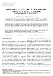
THE PROCESS OF SAFE SHIP’S STEERING The challenge in research for effective methods to prevent ship’s collisions has become imminent with increasing sizes, speeds and number of ships participating in sea cargo carriage. An obvious contribution in increasing safety of shipping has been firstly the application of radars and then the development of an anti-collision system ARPA (Automatic Radar Plotting Aids) [3,4,5]. The ARPA system enables to automatically track at least j=20 objects encountered, to determine their movement parametres (speed Vj and course ψj) and elements indicating their closing to the own ship (DCPAj Distance of the Closest Point of Approach, T CPAj - Time to the Closest Point of Approach) together with the risk of collision (Fig.1).
ABSTRACT The article presents the application of an artificial neural network in anti-collision systems at sea. The systems determine safe trajectory for a ship by processing the information sourced from an ARPA (Automatic Radar Plotting Aids) type arrangement. In this research work the use of neural classifier has been proposed as an element supporting a navigator in the process of determining the ship’s domain, i.e. the area around a ship which, for safety reasons, should remain free from navigational obstacles. Neural classifier has a form of a multilayer feedforward network of a perceptronic nature. It has been assigned a task to represent the evaluation of a navigational situation provided by an experienced navigator functioning as a teacher in the process of the network learning phase. Programs designed in the MATLAB language have been applied for the simulation of the network and also for the illustration of a navigational situation. Testing of the correctness of classification of the collision situations by the network have been also conducted. In the final part of the article conclusions have been formulated with regard to the application of the neural classifier in the process of determining a safe trajectory of a ship.
INTRODUCTION According to the Lloyd’s data the volume of the tonnage lost as a result of collisions sustained by vessels in proportion to all losses sustained as a result of sinking, fire, missing or shipwreck varies depending on a year from a few up to a dozen or so percent. It is assumed that approximately half of the losses may be avoided using better methods of comprehensively supported safe steering of the ship’s movement, specially when latest methods of modern theory of automatic steering are applied such as: differential games, fuzzy control, expert systems, neural networks, genetic algorithms, etc. [6,7,8].
Fig. 1. The process of a safe passing of the own ship with a “j” number of ships encountered.
However, the operational range of a standard ARPA system ends up with the simulation of a manoeuvre selected by navigator. The problem of choosing such a manoeuvre is very difficult. Navigator makes a decision on the type of manoeuvre to avoid collision considering the information originated from ARPA system and also basing on his experience and intuition. One of the factors taken under consideration by a navigator is the ship’s domain i.e. the area surrounding a ship within which, for safety reasons, no other vessels or navigational obstructions should be found. The ship’s domain is defined by the operator of the anticollision system on the basis of the numerical information provided by the navigational devices and by the measuring systems installed on board a ship together with the use of the navigator’s subjective feelings regarding the degree of threat of a collision under the analysed navigational situation.
In practice the methods of choosing a manoeuvre assume a form of appropriate steering algorithms programmed in the memory of a microprocessor controller constituting an option within the ARPA anticollision system or a simulator found at a laboratory of a maritime college [10,14]. The manner in which a ship, being a multi-dimensional and non-linear dynamic object, is steered depends on the extent and precision of the information on current navigational situation and also on the adopted model for the process [11,13]. During its development it is crucial to take into account the following: kinematic and dynamic equations of the own ship interference generated by the sea motion and interaction of wind and sea current, strategy of the objects encountered, function of the steering target, etc. (Fig. 2).
THE NEURAL MODEL OF SHIP’S DOMAIN ASSESSMENT One of the fundamental features of multi-layer, feedforward neural networks, is their ability to represent any u vector given at the network input in the form of an y output vector [7]. The form of representation is formulated through the network topology and through the values of the weigh coefficients given at the input of particular neurons. Teaching the network proceeds through the tuning of the weigh coefficient values in such a way so that for any given input vector (also referred to as image or input pattern) the response at the network output is as near the output pattern presented by the teacher as possible. Thus this is a heteroassociative type of learning [5]. Therefore the following equation: Y = F(U)
(1)
where: U – set of input vectors, Y - set of corresponding output vectors, represented by a trained network need not be previously given in the form of a known analytic relationship. It may be a representation of a heuristic knowledge of the operator who prepares relevant sets of the input images and their corresponding “reasonable” responses. Let us consider then a network with five inputs and one output. The task given to the network will be to assign one of the accepted values of the response to each specific input vectors with the smallest error possible. Fig. 2. Block diagram of the models for steering
process: U - vector of the own ship steering,
U
j
steering vector of the “j” ship, X - state vector of the “j”
yk = F(uk)
(2)
uk = [Njk, Vjk, Vk, jk, Djk]
(3)
ydk < 0.1 0.3 0.5 0.7 0.9 >
(4)
-
ship, Z - disturbance vector, R - vector of safety the situation (risk of collision).
Therefore we are seeking: A wide variety of models possible to be adopted directly influences the synthesis of various steering algorithms and consequently on the effects of safe control of the own ship’s movements (Fig.3).
Fig.3. The structure of a system of safe steering a ship.
min [ F
(y
k
y dk ) 2 ]
(5)
where: y – response of the network, ydk required response by the network, F mapping presented by the network, Nj bearing to a ”j” ship, Vj speed of a ”j” ship, V – speed of the own ship, j relative course of a ”j” ship, Dj distance between own ship and ”j” ship, k – index of a time moment. The values of the element of uk vector are provided from ARPA system and the yk values determine a degree of a collision threat. Such a network is illustrated in Figure 4. The network has three layers of neurons. The non-linear functions of activation in the first and the second layer are of hyperbolic tangent (bipolar) nature and in the output layer the functions have a log-sigmoid (unipolar) nature.
The network has been modelled with the use of Neural Network Toolbox from the MATLAB package. The process of learning used a backpropagation algorithm with adaptively matched learning rate and momentum [7]. NBj
f
f
f
f
Vj
V
.. .
j
.. .
y
f Output Layer
DABj W1jk
f
Input Layer
W2kl
f
W3lm
Hidden Layer
Fig. 4. Structure of neural network used for navigator’s knowledge representation. Figure 5 shows an example of a record for an error function of the network during its learning process. The achievement of a required error level mainly depends on the coherence of data used at the learning stage. While preparing the learning patterns navigator, guided by his own subjective impressions, may assess two very similar navigational situations in a different manner. The network then may generate incorrect responses if the input signal vectors from the testing pattern are close enough to the learning vector with which an answer not identical in meaning is associated. The coherence of data may be improved by presenting navigator a few times the same data in a different sequence and rejecting responses which do not repeat. The results of experiments also indicate the necessity to interfere in dissipating of the patterns used during the learning process of the network in the space of all possible navigational situations. Condensation of input vectors considered in the vicinity of the hyper plane dividing this space into the “safe” and “unsafe” parts fundamentally reduces the number of incorrect responses of the network.
Z =
(6)
Figure 6 illustrates one of the examples presented to the navigator. The collected data are saved in the sets in a format enabling to use them directly by the m-files of the Neural Network Toolbox.
15
10
5
n.m
0
-5
-10
N 33 e 1 t 10 w o r 0 k 10
-15 -15 COLLISION!
E -1 r 10 r o r -2 10
0
-10
-5 v=5.007
n.m. 0 vj=14.3308
5 Pattern No19
10
15
of 200
Fig. 6. Example of navigational situation presented to the navigator.
0,009
-3
10
One of the fundamental problems in teaching the network is preparation of the input data sets and, corresponding to them, required output data. These data should be coherent and evenly cover the space of possible inputs of the network [14]. In order to collect appropriate teaching data a MATLAB m-file has been programmed presenting a selected navigational situation to an experienced navigator. The parameters of the ship’s movement are presented on the screen in the form of vectors, similarly to the way parameters are displayed on the ARPA screen. It has been assumed that the radius of the largest circle of observation is 15 n.m. The responding person may express his/her assessment of the presented situation by clicking the mouse on to one of the proposed answers. In the currently presented version, the program memorises one out of five possibilities. As a result of this a set of input and output values is being generated in the following form:
1000
2000 3000 Epoch s
4000
5000
Fig.5. Network sum squared error in learning process.
Each of the particular required values of the network outputs, a description available to the navigator performing a function of an expert has been assigned. This has been illustrated in Table 1.
Tab.1. The description of the network outputs. ydk
Description
0.1
Safe situation
0.3
Attention
0.5
Threat
0.7
Situation decidedly dangerous
0.9
Collision
process model. For this reason the assigning of a ship trajectory in a collision situation represents a standard dynamic optimization problem with constraints, which can be solved with the help of the Pontriagin’s maximum principle or the Bellman’s dynamic programming. The dynamic programming method seems to be most adequate for the determining safe ship’s optimal course and speed in collision situation [1,2,5,12]. Let us assume that the Tk time of ship’s motion on any path from the point (x10,x20) at t0 instant up to the point
(t1k,t2k) at the tk instanty, whilst the T k is equal to the optimal (minimum) motion time between the above points, then the K stages trajectory total time equals:
SIMULATION RESULTS The results of teaching the network have been used during the simulation of a situation when own-ship encounters three other ships. Domains have been drawn around target ships that serve to provide data on dangerous areas for the anti-collision system of own ship. All ships were moving along rectilinear courses. Figure 7 illustrates successive stages of the changes in the target ship domain when the said ship is passing along the starboard of the own-ship from the bow sector at a speed of 12 knots. The ship’s domain clearly decreases after passing on to the stern sector and proportionally to the increasing distance from the ownship.
Tk min[Tk1 ( x10 , x 20 , t 0 , x1,k 1, x 2,k 1, t k 1 ) k ,Vk
(7)
t k ( k , Vk , x1,k 1 , x 2,k 1, t k 1 )] The trajectory time tk can be expressed as follows:
t k
z k (x 1,k 1, x 2,k 1, t k 1, x 1k , x 2k , t k ) Vk
(8)
where: zk – the route from (x1,k-1,x2,k-1) point up to the (x1k,x2k) point, Vk – the own ship speed at the k stage (Fig.8).
30
20
10
Mm
0
-10
-20
Fig.8. The division of ship’s itinerary into K stages. -30 -30
-20
-10
0 Mm
10
20
30
Fig. 7. Simulation results of ship passing along the starboard. DETERMINING THE SAFE SHIP’S OPTIMAL TRAJECTORY The above formulated ship’s domain determines the constraints of the control and state variables in the
The formula (7) represents the Bellman’s functional equation for the steering process of a ship by speed and course change in collision situation. The state variables constraints formulated as ship’s domain by neural network are entering in the computer program as separate procedure recorded in CONSTR mathematical symbol. The trajectories have been computed for each simulated situation both for a good and a restricted visibility at the sea. The results have been compared by performing the
manoeuvres with the steering course and speed or only the course alternations (Fig.9).
REFERENCES [1] E.Angel, R.Bellman, ”Dynamic programming and partial differential equations”, Academic Press,1972 [2] R.Bellman, ”Introduction to matrix analysis”, London, 1960 [3] B. A. Colley, R. G. Curtis, C. T. Stockel, ” Manoeuvring times, domains and areas”, Journal of Navigation, No. 36, 1983, pp. 324-328 [4] P.V. Davis, M..J. Dove, C.T. Stockel, ” A computer simulation of marine traffic using domains and areas”, Journal of Navigation, No.33, 1980, pp. 215-222 [5] R.C. Dorf, R.H. Bishop, ”Modern control systems”, Addison Wesley Publ., 1998, pp.641-752 [6] E.M. Goodwin, ”A statistical study of ship domains”, Journal of Navigation, No.28, 1975, pp. 328334
Fig.9. Time optimal ship’s safe trajectories in the situation passing of 20 met objects: —— good visibility, Db=0.5 nm, manoeuvring by course and speed change, T=1.0270 h, ----- restricted visibility, Db=3.0 nm, manoeuvring by course and speed change, T=1.4152 h, ........ restricted visibility, D b=3.0 nm, manoeuvring by course change only, T =2.123 h.
CONCLUSIONS The neural networks presented in this article may be applied as elements of the systems used for the assessment of safety when ships are passing one another by the introduction of a possibility to make prompt corrections to the extents of the ships’ domains. They are able to represent a heuristic knowledge similar to an experienced navigator’s knowledge. The correctness of the assessment of the passing ships with the use of the network depends, to a decisive degree, on the correctness of the data used in the process of teaching the network. The use of the knowledge of a few experienced navigators during the teaching process may lead to the fact that the network may enjoy “averaged” knowledge. The introduction of an element of artificial intelligence which exists within an appropriately prepared neural network into the systems of determining the ship’s domain and, as a consequence, possibility to determine her safe trajectory under a collision situation may be of assistance to a less experienced navigator supervising the anti-collision system when assessing the navigational situation, may increase the safety of an anti-collision manoeuvre and also accelerate the process of deciding on the manoeuvre leading to the avoidance of a collision.
[7] J.Hertz, A. Krogh, R.G.Palmer, ”Introduction to the theory of neural computation”, Addison Wesley Publ., 1991 [8] K.J. Hunt, G.R. Irwin, K. Warwick, ”Neural network engineering in dynamic systems”, Advances in industrial control, Springer, 1998 [9] IMO, ”Preference Standards for Automatic Radar Plotting Aids (ARPA)”, Resolution A. 422 (XI), Nov. 1979 [10] C.T.Leondes, ”Control and dynamic systems”, Neural network systems techniques and applications, Vol.7, Academic Press, 1998 [11] J.Lisowski, ”Ship’s anticollision systems”, Wydawnictwo Morskie, Gdańsk, 1981 (In Polish) [12] J.Lisowski, ”Determining of optimal safe ship’s trajectory using dynamic programming method”, Scientific Journal of Gdynia Maritime Academy, No.20, Gdynia, 1990 pp.16-29 (In Polish) [13] J.Lisowski, A. Rak, A. Grzenia, ”Neural classification of dangerous ships in collision situations”, Proc. of IMACS/IFAC International Symposium on Soft Computing in Engineering Applications, SOFTCOM’98, Athens, Greece, 1998 [14] R.Tadeusiewicz, ”Neural Networks”, Akademicka Oficyna Wydawnicza RM, Warszawa, 1993 (In Polish)