The Bayesian occupation filter

Author manuscript, published in "Probabilistic Reasoning and Decision Making in Sensory-Motor Systems, Bessière, P. and Laugier, C. and Siegwart, R. (Ed.) (2008)"

The Bayesian occupation filter M.K Tay1 , K. Mekhnacha2 , M. Yguel1 , C. Coué1 , C. Pradalier3 , C. Laugier1 Th. Fraichard1 and P. Bessière4 1 2 3 4

INRIA Rhône-Alpes PROBAYES CSIRO ICT Centre, Queensland Centre for Advanced technologies (QCAT) CNRS - Grenoble Université

inria-00295084, version 1 - 11 Jul 2008

1 Introduction Perception of and reasoning about dynamic environments is pertinent for mobile robotics and still constitutes one of the major challenges. To work in these environments, the mobile robot must perceive the environment with sensors; measurements are uncertain and normally treated within the estimation framework. Such an approach enables the mobile robot to model the dynamic environment and follow the evolution of its environment. With an internal representation of the environment, the robot is thus able to perform reasoning and make predictions to accomplish its tasks successfully. Systems for tracking the evolution of the environment have traditionally been a major component in robotics. Industries are now beginning to express interest in such technologies. One particular example is the application within the automotive industry for adaptive cruise control [Coué et al., 2002], where the challenge is to reduce road accidents by using better collision detection systems. The major requirement of such a system is a robust tracking system. Most of the existing target-tracking algorithms use an object-based representation of the environment. However, these existing techniques must explicitly consider data association and occlusion. In view of these problems, a gridbased framework, the Bayesian occupancy filter (BOF) [Coué et al., 2002, 2003], has been proposed. 1.1 Motivation In classical tracking methodology [Bar-Shalom and Fortman, 1988], the problem of data association and state estimation are major problems to be addressed. The two problems are highly coupled, and an error in either component leads to erroneous outputs. The BOF makes it possible to decompose this highly coupled relationship by avoiding the data association problem, in the sense that the data association is handled at a higher level of abstraction.

inria-00295084, version 1 - 11 Jul 2008

80

M.K Tay , K. Mekhnacha, M. Yguel, C. Coué, C. Pradalier, et al.

In the BOF model, concepts such as objects or tracks do not exist; they are replaced by more useful properties such as occupancy or risk, which are directly estimated for each cell of the grid using both sensor observations and some prior knowledge. It might seem strange to have no object representations when objects obviously exist in real life environments. However, an object-based representation is not required for all applications. Where object-based representations are not pertinent, we argue that it is more useful to work with a more descriptive, richer sensory representation rather than constructing object-based representations with their complications in data association. For example, to calculate the risk of collision for a mobile robot, the only properties required are the probability distribution on occupancy and velocities for each cell in the grid. Variables such as the number of objects are inconsequential in this respect. This model is especially useful when there is a need to fuse information from several sensors. In standard methods for sensor fusion in tracking applications, the problem of track-to-track association arises where each sensor contains its own local information. Under the standard tracking framework with multiple sensors, the problem of data association will be further complicated: as well as the data association between two consecutive time instances from the same sensor, the association of tracks (or targets) between the different sensors must be taken into account as well. In contrast, the grid-based BOF will not encounter such a problem. A gridbased representation provides a conducive framework for performing sensor fusion [Moravec, 1988]. Different sensor models can be specified to match the different characteristics of the different sensors, facilitating efficient fusion in the grids. The absence of an object-based representation allows easier fusing of low-level descriptive sensory information onto the grids without requiring data association. Uncertainty characteristics of the different sensors are specified in the sensor models. This uncertainty is explicitly represented in the BOF grids in the form of occupancy probabilities. Various approaches using the probabilistic reasoning paradigm, which is becoming a key paradigm in robotics, have already been successfully used to address several robotic problems, such as CAD modelling [Mekhnacha et al., 2001] and simultaneous map building and localization (SLAM) [Thrun, 1998, Kaelbling et al., 1998, Arras et al., 2001]. In modelling the environment with BOF grids, the object model problem is nonexistent because there are only cells representing the state of the environment at a certain position and time, and each sensor measurement changes the state of each cell. Different kinds of objects produce different kinds of measures, but this is handled naturally by the cell space discretization. Another advantage of BOF grids is their rich representation of dynamic environments. This information includes the description of occupied and hidden areas (i.e. areas of the environment that are temporarily hidden to the sensors by an obstacle). The dynamics of the environment and its robustness relative to object occlusions are addressed using a novel two-step mechanism

The Bayesian occupation filter

81

that permits taking the sensor observation history and the temporal consistency of the scene into account. This mechanism estimates, at each time step, the state of the occupancy grid by combining a prediction step (history) and an estimation step (incorporating new measurements). This approach is derived from the Bayesian filter approach [Jazwinsky, 1970], which explains why the filter is called the Bayesian occupancy filter (BOF). The five main motivations in the proposed BOF approach are as follows. •

inria-00295084, version 1 - 11 Jul 2008

•

•

•

•

Taking uncertainty into account explicitly, which is inherent in any model of a real phenomenon. The uncertainty is represented explicitly in the occupancy grids. Avoiding the “data association problem” in the sense that data association is to be handled at a higher level of abstraction. The data association problem is to associate an object ot at time t with ot+1 at time t+1. Current methods for resolving this problem often do not perform satisfactorily under complex scenarios, i.e. scenarios involving numerous appearances, disappearances and occlusions of several rapidly manoeuvring targets. The concept of objects is nonexistent in the BOF and hence avoids the problem of data association from the classical tracking point of view. Avoiding the object model problem, that is, avoiding the need to make assumptions about the shape or size of the object. It is complex to define what the sensor could measure without a good representation of the object. In particular, a big object may give multiple detections whereas a small object may give just one. In both cases, there is only one object, and that lack of coherence causes multiple-target tracking systems, in most cases, to work properly with only one kind of target. An Increased robustness of the system relative to object occlusions, appearances and disappearances by exploiting at any instant all relevant information on the environment perceived by the mobile robot. This information includes the description of occupied and hidden areas (i.e. areas of the environment that are temporarily hidden to the sensors by an obstacle). A method that could be implemented later on dedicated hardware, to obtain both high performance and decreased cost of the final system.

1.2 Objectives of the BOF We claim that in the BOF approach, the five previous objectives are met as follows. • • •

Uncertainty is taken into account explicitly, thanks to the probabilistic reasoning paradigm, which is becoming a key paradigm in robotics. The data association problem is postponed by reasoning on a probabilistic grid representation of the dynamic environment. In such a model, concepts such as objects or tracks are not needed. The object model problem is nonexistent because there are only cells in the environment state, and each sensor measurement changes the state of each

82

•

•

M.K Tay , K. Mekhnacha, M. Yguel, C. Coué, C. Pradalier, et al.

cell. The different kinds of measures produced by different kinds of object are handled naturally by the cell space discretization. The dynamics of the environment and its robustness relative to object occlusions are addressed using a novel two-step mechanism that permits taking the sensor observation history and the temporal consistency of the scene into account. The Bayesian occupancy filter has been designed to be highly parallelized. A hardware implementation on a dedicated chip is possible, which will lead to an efficient representation of the environment of a mobile robot.

This chapter presents the concepts behind BOF and its mathematical formulation, and shows some of its applications.

inria-00295084, version 1 - 11 Jul 2008

• • • • •

Section 2 introduces the basic concepts behind the BOF. Section 2.1 introduces Bayesian filtering in the 4D occupancy grid framework [Coué et al., 2006]. Section 2.2 describes an alternative formulation for filtering in the 2D occupancy grid framework [Tay et al., 2007]. Section 3 shows several applications of the BOF. Section 4 concludes this chapter.

2 Bayesian occupation filtering The consideration of sensor observation history enables robust estimations in changing environments (i.e. it allows processing of temporary objects, occlusions and detection problems). Our approach for solving this problem is to make use of an appropriate Bayesian filtering technique called the Bayesian occupancy filter (BOF). Bayesian filters Jazwinsky [1970] address the general problem of estimating the state sequence xk , k ∈ N of a system given by: xk = f k (xk−1 , uk−1 , wk ),

(1)

where f k is a possibly nonlinear transition function, uk−1 is a “control” variable (e.g. speed or acceleration) for the sensor that allows it to estimate its own movement between time k − 1 and time k, and wk is the process noise. This equation describes a Markov process of order one. Let z k be the sensor observation of the system at time k. The objective of the filtering is to estimate recursively xk from the sensor measurements: z k = hk (xk , v k )

(2)

where hk is a possibly nonlinear function and v k is the measurement noise. This function models the uncertainty of the measurement z k of the system’s state xk .

The Bayesian occupation filter

83

inria-00295084, version 1 - 11 Jul 2008

In other words, the goal of the filtering is to estimate recursively the probability distribution P (X k | Z k ), known as the posterior distribution. In general, this estimation is done in two stages: prediction and estimation. The goal of the prediction stage is to compute an a priori estimate of the target’s state known as the prior distribution. The goal of the estimation stage is to compute the posterior distribution, using this a priori estimate and the current measurement of the sensor. Exact solutions to this recursive propagation of the posterior density do exist in a restrictive set of cases. In particular, the Kalman filter [Kalman, 1960, Welch and Bishop] is an optimal solution when the functions f k and hk are linear and the noise values wk and v k are Gaussian. In general, however, solutions cannot be determined analytically, and an approximate solution must be computed.

Prediction

6

Z

?

?

Estimation

Fig. 1. Bayesian occupancy filter as a recursive loop.

In this case, the state of the system is given by the occupancy state of each cell of the grid, and the required conditions for being able to apply an exact solution such as the Kalman filter are not always verified. Moreover, the particular structure of the model (occupancy grid) and the real-time constraint imposed on most robotic applications lead to the development of the concept of the Bayesian occupancy filter. This filter estimates the occupancy state in two steps, as depicted in Fig. 1. In this section, two different formulations of the BOF will be introduced. The first represents the state space by a 4-dimensional grid, in which the occupancy of each cell represents the joint space of 2D position and 2D velocity. The estimation of occupancy and velocity in this 4D space are described in Section 2.1. The second formulation of the BOF represents the state space by a 2dimensional occupancy grid. Each cell of the grid is associated with a probability distribution on the velocity of the occupancy associated with the cell. The differences between the two formulations are subtle. Essentially, the 4D formulation permits overlapping objects with different velocities whereas the

84

M.K Tay , K. Mekhnacha, M. Yguel, C. Coué, C. Pradalier, et al.

2D formulation does not allow for overlapping objects. The estimation on velocity and occupancy in this 2D grid are described in Section 2.2. 2.1 The 4D Bayesian occupation filter

inria-00295084, version 1 - 11 Jul 2008

The 4-dimensional BOF takes the form of a gridded histogram with two dimensions representing positions in 2D Cartesian coordinates and the other two dimensions representing the orthogonal components of the 2-dimensional velocities of the cells. As explained previously in Section 2, the BOF consists of a prediction step and an estimation step in the spirit of Bayesian filtering. Based on this approach, the evolution of the BOF at time k occurs in two steps: 1. the prediction step makes use of both the result of the estimation step at time k −1 and a dynamic model to compute an a priori estimate of the grid; and 2. the estimation step makes use of both this prediction result and the sensor observations at time k to compute the grid values. The next two subsections will explain the prediction and estimation steps of the 4D BOF respectively. Estimation in the 4D BOF The estimation step consists of estimating the occupancy probability of each cell of the grid, using the last set of sensor observations. These observations represent preprocessed information given by a sensor. At each time step, the sensor is able to return a list of detected objects, along with their associated positions and velocities in the sensor reference frame. In practice, this set of observations could also contain two types of false measurements: false alarms (i.e. when the sensor detects a nonexistent object) and missed detections (i.e. when the sensor does not detect an existing object). Solving the static estimation problem can be done by building a Bayesian program. The relevant variables and decomposition are as follows. • • • •

C k : The cell itself at time k; this variable is 4-dimensional and represents a position and a speed relative to the vehicle. k EC : The state of the cell C at time k; whether it is occupied. Z: The sensor observation set; one observation is denoted by Zs , and the number of observation is denoted by S; each variable Zs is 4-dimensional. M : The “matching” variable; it specifies which observation of the sensor is currently used to estimate the state of a cell.

The decomposition of the joint distribution of these variables can be expressed as:

The Bayesian occupation filter k k P (C k EC Z M) = P (C k )P (EC | C k )P (M ) ×

S Y

s=1

85

k P (Zs | C k EC M)

Parametric forms can be assigned to each term of the joint probability decomposition. • • •

inria-00295084, version 1 - 11 Jul 2008

•

P (C k ) represents the information on the cell itself. As we always know the cell for which we are currently estimating the state, this distribution may be left unspecified. k P (EC | C) represents the a priori information on the occupancy of the cell. The prior distribution may be obtained from the estimation of the previous time step. P (M ) is chosen uniformly. It specifies which observation of the sensor is used to estimate the state of a cell. k The shape of P (Zs | C k EC M ) depends on the value of the matching variable. – If M 6= s, the observation is not taken from the cell C. Consequently, k we cannot say anything about this observation. P (Zs | C k EC M ) is defined by a uniform distribution. k – If M = s, the form of P (Zs | C k EC M ) is given by the sensor model. Its goal is to model the sensor response knowing the cell state. Details on this model can be found in Elfes [1989].

It is now possible to ask the Bayesian question corresponding to the searched solution. Because the problem to solve consists of finding a good estimate of the cell occupancy, the question can be stated as the probability distribution on the state of cell occupancy, conditioned on the observations and the cell itself: k P (EC | Z Ck) (3) The result of the inference can be written as: k P (EC

k

|Z C )∝

S X

M=1

S Y

s=1

P (Zs |

k EC

k

!

C M) .

(4)

During inference, the sum on these variables allows every sensor observation to be taken into account during the update of the state of a cell. It should be noted that the estimation step is performed without any explicit association between cells and observations; this problematic operation is replaced by the integration on all the possible values of M . Figure 2 shows the estimation step expressed as a Bayesian program. Prediction in the 4D BOF The goal of this processing step is to estimate an a priori model of the occupancy probability at time k of a cell using the latest estimation of the occupancy grid, i.e. the estimation at time k − 1.

M.K Tay , K. Mekhnacha, M. Yguel, C. Coué, C. Pradalier, et al.

inria-00295084, version 1 - 11 Jul 2008

8 > > > > > > > > > > > > > > > > > > > > > > > > > > > > > > > > > > > > >
> > > C k T he cell itself at time k; this variable is 4-dimensional and > > > > represents a position and a speed relative to the vehicle. > > > k > > E The state of the cell C, occupied or not. C > > > > Z The sensor observation set: one observation is denoted Zs ; > > > > the number of observation is denoted S; > > > > each variable Zs is 4-dimensional. > > > > M The “matching” variable; its goal is to specify which > > > > observation of the sensor is currently used to estimate the < state of a cell. > > Decomposition: > > > > k > > P (C k EC Z M) = > > > > > > > > S > > Q > > > k k k > > > > > P (C )P (EC | C k )P (M ) × P (Zs | C k EC M) > > > > > > > > s=1 > > > > > > > > > > > Parametric Forms: > > > > > > > > > > > > P (C k ): uniform; > > > > > > > > > > > > P (EC k | C k ): from the prediction; > > > > > > > > > > > > P (M ): uniform; > > > > > > : > > k > > P (Zs | C k EC M ): sensor model; > > > > > > > > Identification: > > > > : > > None > > > > Question: > > : k | Z Ck) P (EC 8 > > > > > > > > > > > > > > > > > > > > > > > > > > > > > > > > > > > > > > > > > > > > > > > > > > > > > > > > > > > > > > > > > > > > > > > > > > >
> > > C k Cell C considered at time K > > > k > EC State of cell C at time K > > > k−1 > C Cell C at time k − 1 > > > k−1 > > EC State of cell C at time k − 1 > > > > U k−1 “control” input of the CyCab at time k − 1. For > > > > example, it could be a measurement of its instantaneous > > > > velocity at time k − 1. > > < Decomposition: k−1 k P (C k EC C k−1 EC U k−1 ) = > > > k−1 k−1 k−1 > ) × P (U ) × P (EC | C k−1 ) > P (C > > > > > k−1 k k−1 k−1 k > > > > > | EC C k−1 C k ) ×P (C | C U ) × P (E C > > > > > > > > > > > > Parametric Forms: > > > > > > > > > > > > P (C k−1 ): uniform; > > > > > > > > > > > > P (U k−1 ): uniform; > > > > > > > > > k−1 > > > P (EC | C k−1 ): estimation at time k-1; > > > > > > > > > k k−1 > > > > P (C | C U k−1 ): dynamic model; > > > > > : > > k−1 k > > > > P (EC | EC C k−1 C k ): dirac; > > > > > > > > Identification: > > : > > > None > > > > Question: > : k P (EC | C k U k−1 ) 8 > > > > > > > > > > > > > > > > > > > > > > > > > > > > > > > > > > > > > > > > > > > > > > > > > > > > > > > > > > > > > > > > > > > > > > > > > > > > > > > > > > > > >
> > > > > > > > > > > > > > > > > > > > > > > > > > > > > > > > > > > > > > >
> >C > An index that identifies each 2D cell of the grid. > > > > A An index that identifies each possible antecedent of the cell > > > > c over all the cells in the 2D grid. > > > > Z The sensor measurement relative to the cell c. t > > > > The set of velocities for the cell c where >V > > > V is discretized into n values; V ∈ V = {v1 , . . . , vn }. > > > O, O−1 Takes values from the set O ≡ {occ, emp}, > > > > > indicating whether the cell c is ‘occupied’ or ‘empty’. > > > > O−1 represents the random variable of the state of an < antecedent cell of c through the possible motion through c. > > Decomposition: > > > > > > > P (C A Z O O−1 V ) = > > > > > > > P (A)P (V |A)P (C|V, A)P (O−1 |A)P (O|O−1 )P (Z|O, V, C) > > > > > > > > > > > > > > Parametric Forms: > > > > > > > > > > > > > P (A): uniform; > > > > > > > > > > > > P (V | A): conditional velocity distribution of antecedent cell; > > > > > > > > > > > > P (C | V A): Dirac representing reachability; > > > > > > > > > > P (O−1 | A): conditional occupancy distribution of the antecedent cell; > > > > > > > > > > −1 > > > > > > > : P (O | O ): occupancy transitional matrix; > > > > > > P (Z | O V C): observation model; > > > > > > > > Identification: > > : > > > None > > > > Question: > > > > P (O | Z C) > > : P (V | Z C) Description

Program

The Bayesian occupation filter

Fig. 5. BOF with Velocity Inference

Filtering computation and representation for the 2D BOF The aim of filtering in the BOF grid is to estimate the occupancy and grid velocity distributions for each cell of the grid, P (O, V |Z, C). Figure 6 shows how Bayesian filtering is performed in the 2D BOF grids. The two stages of prediction and estimation are performed for each iteration. In the context of the BOF, prediction propagates cell occupation probabilities for each velocity and cell in the BOF grid (P (O, V |C)). During estimation, P (O, V |C) is updated by taking into account its observation P (Z|O, V, C) to obtain its final Bayesian filter estimation P (O, V |Z, C). The result from the Bayesian filter estimation is then used for prediction in the next iteration. From Fig. 6, the difference between the 2D BOF and the 4D BOF is clearly illustrated. First, the 2D BOF defines the velocity of the cell occupation as a variable in the Bayesian program. The velocity is not expressed as a variable in the Bayesian program in the 4D BOF, but it is rather defined as a prior dynamic model to be given P (C k | C k−1 U k−1 ) (Fig. 3). The 2D BOF is thus

92

M.K Tay , K. Mekhnacha, M. Yguel, C. Coué, C. Pradalier, et al.

Observation P(Z|O,V,C) Prediction P(O,V|C) Estimation P(O,V|Z,C)

inria-00295084, version 1 - 11 Jul 2008

Fig. 6. Bayesian filtering in the estimation of occupancy and velocity distribution in the BOF grids.

capable of performing inference on both the occupation and the velocity of the cell’s occupation. Second, the 2D BOF inherently expresses the constraint of a single occupation and velocity for each cellular decomposition of the 2D Cartesian space. However, in the 4D BOF, there is the possibility of expressing occupation of a cell in 2D Cartesian space with different velocities. The reduction in complexity from four dimensions to two reduces the computational complexity. When implementing the 2D BOF, the set of possible velocities is discretized. One way of implementing the computation of the probability distribution is in the form of histograms. The following equations are based on the discrete case. Therefore, the global filtering equation can be obtained by: P

P (V, O|Z, C) = P

A,O−1

P (C, A, Z, O, O−1 , V )

A,O,O−1 ,V

P (C, A, Z, O, O−1 , V )

,

(8)

which can be equivalently represented as:   X P (V, O, Z, C) = P (Z|O, V, C)  P (A)P (V |A)P (C|V, A)P (O−1 |A)P (O|O−1 ) . A,O−1

The summation in the above expression represents the prediction; its multiplication with the first term, P (Z|O, V, C), gives the Bayesian filter estimation. The global filtering equation (eqn. 8) can actually be separated into three stages. The first stage computes the prediction of the probability measure for each occupancy and velocity:

The Bayesian occupation filter

X

α(occ, vk ) =

A,O−1

X

α(emp, vk ) =

A,O−1

93

P (A)P (vk |A)P (C|V, A)P (O−1 |A)P (occ|O−1 ), P (A)P (vk |A)P (C|V, A)P (O−1 |A)P (emp|O−1 ). (9)

inria-00295084, version 1 - 11 Jul 2008

Equation 9 is performed for each cell in the grid and for each velocity. Prediction for each cell is calculated by taking into account the velocity probability and occupation probability of the set of antecedent cells, which are the cells with a velocity that will propagate itself in a certain time step to the current cell. With the prediction of the grid occupancy and its velocities, the second stage consists of multiplying by the observation sensor model, which gives the unnormalized Bayesian filter estimation on occupation and velocity distribution: β(occ, vk ) = P (Z|occ, vk )α(occ, vk ), β(emp, vk ) = P (Z|emp, vk )α(emp, vk ). Similarly to the prediction stage, these equations are performed for each cell occupancy and each velocity. The marginalization over the occupancy values gives the likelihood of a certain velocity: l(vk ) = β(occ, vk ) + β(emp, vk ). Finally, the normalized Bayesian filter estimation on the probability of occupancy for a cell C with a velocity vk is obtained by: β(occ, vk ) . P (occ, vk |Z, C) = P vk l(vk )

(10)

The occupancy distribution in a cell can be obtained by the marginalization over the velocities and the velocity distribution by the marginalization over the occupancy values: P (O|Z, C) =

X

P (V, O|Z, C),

(11)

P (V, O|Z, C).

(12)

V

P (V |Z, C) =

X O

3 Applications The goal of this section is to show some examples of applications using BOF5 . Two different experiments are shown. The first is on estimating collision dan5

Different videos ing URLs:

of these applications may be found at the followhttp://www.bayesian-programming.org/spip.php?article143,

94

M.K Tay , K. Mekhnacha, M. Yguel, C. Coué, C. Pradalier, et al.

ger, which is in turn used for collision avoidance. The 4D BOF was used for the first experiment. The second is on object-level human tracking using a camera and was based on the 2D BOF. 3.1 Estimating danger

inria-00295084, version 1 - 11 Jul 2008

The experiments on danger estimation and collision avoidance were conducted using the robotic platform CyCab. CyCab is an autonomous robot fashioned from a golf cab. The aim of this experiment is to calculate the danger of collision with dynamic objects estimated by the BOF, followed by a collision avoidance manoeuvre. The cell state can be used to encode some relevant properties of the robot environment (e.g. occupancy, observability and reachability). In the previous sections, only the occupancy characteristic was stored; in this application, the danger property is encoded as well. This will lead to vehicle control by taking occupancy and danger into account. 10

8

6

4

2

0

4

2

0

-2

-4

Fig. 7. Cells with high danger probabilities. For each position, arrows model the speed.

For each cell of the grid, the probability that this cell is hazardous is estimated; this estimation is done independently of the occupancy probability. k Let P (DC | C k ) be the probability distribution associated with the cell C k http://www.bayesian-programming.org/spip.php?article144 http://www.bayesian-programming.org/spip.php?article145

and

The Bayesian occupation filter

95

pedestrian

parked car

Cycab

inria-00295084, version 1 - 11 Jul 2008

Fig. 8. Scenario description: the pedestrian is temporarily hidden by a parked car. k of the vehicle environment, where DX is a boolean variable that indicates whether this cell is hazardous or not.

Fig. 9. Snapshots of the experimental pedestrian avoidance scenario (see Extension 1 for the video).

Basically, both “time to collision” and “safe travelling distance” may be seen as two complementary relevant criteria to be used for estimating the danger to associate with a given cell. In our current implementation, we are using the following related criteria, which can easily be computed: (1) the closest point of approach (CPA), which defines the relative positions of the

inria-00295084, version 1 - 11 Jul 2008

96

M.K Tay , K. Mekhnacha, M. Yguel, C. Coué, C. Pradalier, et al.

pair (vehicle, obstacle) corresponding to the “closest admissible distance” (i.e. safe distance); (2) the time to the closest point of approach (TCPA), which is the time required to reach the CP A; and (3) the distance at the closest point of approach (DCPA), which is the distance separating the vehicle and the obstacle when the CP A has been reached. In some sense, these criteria give an assessment of the future relative trajectories of any pair of environment components of the types (vehicle, potential obstacle). These criteria are evaluated for each cell at each time step k, by taking into account the dynamic characteristics of both the vehicle and the potential obstacles. In practice, both T CP A and DCP A are estimated under the hypothesis that the related velocities at time k remain constant; this computation can easily be done using some classical geometrical algorithms (see for instance: http://softsurfer.com/algorithms.htm). The goal is to estimate the “danger probability” associated with each cell of the grid (or in other terms, the probability for each cell C k that a collision will occur in the near future between the CyCab and a potential obstacle in C k ). Because each cell C k represents a pair (position, velocity) defined relative to the CyCab, it is easy to compute the T CP A and DCP A factors, and in a second step to estimate the associated danger probability using given intuitive user knowledge. In the current implementation, this knowledge roughly states that when the DCP A and the T CP A decrease, the related probability of collision increases. In future versions of the system, such knowledge can be acquired with a learning phase. Figure 7 shows the cells for which the danger probability is greater than 0.7 in our CyCab application; in the figure, each cell is represented by an arrow: its tail indicates the position, and its length and direction indicate the associated relative speed. This figure exhibits quite reasonable data: cells located near the front of the CyCab are considered as having a high danger probability for any relative velocity (the arrows are pointing in all directions); the other cells having a high “oriented” danger probability are those having a relative speed vector oriented towards the CyCab. Because we only consider relative speeds when constructing the danger grid, the content of this grid does not depend on the actual CyCab velocity. 3.2 Collision avoidance behaviours This section describes the control of the longitudinal speed of the autonomous vehicle (the CyCab), for avoiding partially observed moving obstacles having a high probability of collision with the vehicle. The implemented behaviour consists of braking or accelerating to adapt the velocity of the vehicle to the level of risk estimated by the system. As mentioned earlier, this behaviour derives from the combination of two criteria defined on the grid: the danger probability associated with each cell k C k of the grid (characterized by the distribution P (DC | C k )), and the occupancy probability of this cell (characterized by the posterior distribution

The Bayesian occupation filter

97

k P (EC | Z k C k )). In practice, the most hazardous cell that is considered as probably occupied is searched for; this can be done using the following equation: k k max {P (DC | C k ), with P (EC | C k ) > 0.5}. Ck

2

Vconsigne (m/s-1)

inria-00295084, version 1 - 11 Jul 2008

Then the longitudinal acceleration/deceleration to apply to the CyCab controller can be decided according to the estimated level of danger and to the actual velocity of the CyCab. Figure 8 depicts the scenario used for experimentally validating the previous collision avoidance behaviour on the CyCab. In this scenario, the CyCab is moving forward, the pedestrian is moving from right to left, and for a small period of time, the pedestrian is temporarily hidden by a parked car. Figure 9 shows some snapshots of the experiment (see also Extension 1, which shows the entire video): the CyCab brakes to avoid the pedestrian, then it accelerates as soon as the pedestrian has crossed the road.

1.5

1

0.5

0 0

2

4

6

8 time (s)

10

12

14

Fig. 10. Velocity of the CyCab during the experiment involving a pedestrian occlusion.

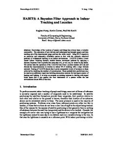
Figure 10 shows the velocity of the CyCab during this experiment. From t = 0 s to t = 7 s, the CyCab accelerates, up to 2 m/s. At t = 7 s, the pedestrian is detected; as a collision could possibly occur, the CyCab decelerates. From t = 8.2 s to t = 9.4 s, the pedestrian is hidden by the parked car; thanks to the BOF results, the hazardous cells of the grid are still considered as probably occupied; in consequence the CyCab still brakes. When the pedestrian reappears at t = 9.4 s, there is no longer a risk of collision, and the CyCab can accelerate. 3.3 Object-level tracking Experiments were conducted based on video sequence data from the European project CAVIAR. The selected video sequence presented in this paper is taken from the interior of a shopping centre in Portugal. An example is shown in the first column of Fig. 11. The data sequence from CAVIAR, which is freely available from the Web6 , gives annotated ground truths for the detection of 6

http://groups.inf.ed.ac.uk/vision/CAVIAR/CAVIARDATA1/

inria-00295084, version 1 - 11 Jul 2008

98

M.K Tay , K. Mekhnacha, M. Yguel, C. Coué, C. Pradalier, et al.

the pedestrians. Another data set is also available, taken from the entry hall of INRIA Rhône Alpes. Based on the given data, the uncertainties, false positives and occlusions have been simulated. The simulated data are then used as observations for the BOF. The BOF is a representation of the planar ground of the shopping centre within the field of view of the camera. With the noise and occlusion by simulated bounding boxes that represent human detections, a Gaussian sensor model is used, which gives a Gaussian occupation uncertainty (in the BOF grids) of the lower edge of the image bounding box after being projected onto the ground plane. Recalling that there is no notion of objects in the BOF, object hypotheses are obtained from clustering, and these object hypotheses are used as observations on a standard tracking module based on the joint probabilistic data association (JPDA). Previous experiments based on the 4D BOF technique (Section 3.1) relied on the assumption of a given constant velocity, as the problem of velocity estimation in this context has not been addressed. In particular, the assumption that there could only be one object with one velocity in each cell was not part of the previous model. In this current experiment, experiments were conducted based on the 2D BOF model, which gives both the probability distribution on the occupation and the probability distribution on the velocity. The tracker is implemented in the C++ programming language without optimizations. Experiments were performed on a laptop computer with an Intel Centrino processor with a clock speed of 1.6 GHz. It currently tracks with an average frame rate of 9.27 frames/s. The computation time required for the BOF, with a grid resolution of 80 cells by 80 cells, takes an average of 0.05 s. The BOF represents the ground plane of the image sequence taken from a stationary camera and represents a dimension of 30 m by 20 m. The results in Fig. 11 are shown in time sequence. The first column of the figures shows the input image with the bounding boxes, each indicating the detection of a human after the simulation of uncertainties and occlusions. The second column shows the corresponding visualization of the Bayesian occupancy filter. The colour intensity of the cells represents the occupation probability of the cell. The little arrows in each cell give the average velocity calculated from the velocity distribution of the cell. The third column gives the tracker output given by a JPDA tracker. The numbers in the diagrams indicate the track numbers. The sensor model used is a 2D planar Gaussian model projected onto the ground. The mean is given by the centre of the lower edge of the bounding box. The characteristics of the BOF can be seen from Fig. 11. The diminished occupancy of a person further away from the camera is seen from the data in Figs. 11(b) and 11(e). This is caused by the occasional instability in human detection. The occupancy in the BOF grids for the missed detection diminishes gradually over time rather than disappearing immediately as it does

inria-00295084, version 1 - 11 Jul 2008

The Bayesian occupation filter

(a)

(b)

(c)

(d)

(e)

(f)

(g)

(h)

(i)

(j)

(k)

(l)

(m)

(n)

(o)

99

Fig. 11. Data sequence from project CAVIAR with simulated inputs. The first column displays camera image input with human detection, the second column displays the BOF grid output, and the third column displays tracking output. Numbers indicate track numbers.

100

M.K Tay , K. Mekhnacha, M. Yguel, C. Coué, C. Pradalier, et al.

with classical occupation grids. This mechanism provides a form of temporal smoothing to handle unstable detection. A more challenging occlusion sequence is shown in the last three rows of Fig. 11. Because of a relatively longer period of occlusion, the occupancy probability of the occluded person becomes weak. However, with an appropriately designed tracker, such problems can be handled at the object tracker level. The tracker manages to track the occlusion at the object tracker level as shown in Fig. 11(i)(l)(o).

4 Conclusion

inria-00295084, version 1 - 11 Jul 2008

In this chapter, we introduced the Bayesian occupation filter, its different formulations and several applications. •

• •

•

• •

The BOF is based on a gridded decomposition of the environment. Two variants were described, a 4D BOF in which each grid cell represents the occupation probability distribution at a certain position with a certain velocity, and a 2D BOF in which the grid represents the occupation probability distribution and each grid is associated with a velocity probability distribution of the cell occupancy. The estimation of cell occupancy and velocity values is based on the Bayesian filtering framework. Bayesian filtering consists of two main steps, the prediction step and the estimation step. The 4D BOF allows representation of several “objects”, each with a distinct velocity. There is also no inference on the velocity for the 4D BOF. In contrast, the 2D BOF implicitly imposes constraints in having only a single “object” occupying a cell, and there is inference on velocities for the 2D BOF framework. Another advantage of the 2D BOF framework over the 4D BOF is the reduction in computational complexity as a consequence of the reduction in dimension. There is no concept of objects in the BOF. A key advantage of this is “avoiding” the data association problem by resolving it as late as possible in the pipeline. Furthermore, the concept of objects is not obligatory in all applications. However, in applications that require object-based representation, object hypotheses can be extracted from the BOF grids using methods such as clustering. A grid-based representation of the environment imposes no model on the objects found in the environment, and sensor fusion in the grid framework can be conveniently and easily performed.

We would like to acknowledge the European project carsense: IST-199912224 “Sensing of Car Environment at Low Speed Driving”, Carsense [January 2000–December 2002] for the work on the 4D BOF [Coué et al., 2006].

The Bayesian occupation filter

101

inria-00295084, version 1 - 11 Jul 2008

References K. Arras, N. Tomatis, and R. Siegwart. Multisensor on-the-fly localization : precision and reliability for applications. Robotics and Autonomous Systems, 44:131–143, 2001. Y. Bar-Shalom and T. Fortman. Tracking and Data Association. Academic Press, 1988. C. Coué, T. Fraichard, P. Bessière, and E. Mazer. Multi-sensor data fusion using bayesian programming: an automotive application. In Proc. of the IEEE-RSJ Int. Conf. on Intelligent Robots and Systems, Lausanne, (CH), Octobre 2002. C. Coué, T. Fraichard, P. Bessière, and E. Mazer. Using bayesian programming for multi-sensor multi-target tracking in automotive applications. In Proceedings of IEEE International Conference on Robotics and Automation, Taipei (TW), septembre 2003. C. Coué, C. Pradalier, C. Laugier, T. Fraichard, and P. Bessière. Bayesian occupancy filtering for multitarget tracking: an automotive application. Int. Journal of Robotics Research, 25(1):19–30, January 2006. A. Elfes. Using occupancy grids for mobile robot perception and navigation. IEEE Computer, Special Issue on Autonomous Intelligent Machines, Juin 1989. A. H. Jazwinsky. Stochastic Processes and Filtering Theory. New York : Academic Press, 1970. ISBN 0-12381-5509. L. Kaelbling, M. Littman, and A. Cassandra. Planning and acting in partially observable stochastic domains. Artificial Intelligence, 101, 1998. R. Kalman. A new approach to linear filtering and prediction problems. Journal of basic Engineering, 35, Mars 1960. K. Mekhnacha, E. Mazer, and P. Bessière. The design and implementation of a bayesian CAD modeler for robotic applications. Advanced Robotics, 15 (1):45–70, 2001. H. Moravec. Sensor fusion in certainty grids for mobile robots. AI Magazine, 9(2), 1988. C. Tay, K. Mekhnacha, C. Chen, M. Yguel, and C. Laugier. An efficient formulation of the bayesian occupation filter for target tracking in dynamic environments. International Journal Of Autonomous Vehicles, To Appear Spring, 2007. (Accepted) To be published. S. Thrun. Learning metric-topological maps for indoor mobile robot navigation. Artificial Intelligence, 99(1), 1998. G. Welch and G. Bishop. An introduction to the Kalman filter. available at http://www.cs.unc.edu/ welch/kalman/index.html.