THE DYNAMIC SIMULATION OF THE THREE-PHASE BRUSHLESS PERMANENT MAGNET AC MOTOR DRIVES WITH LabVIEW Li Ying * and Nesimi Ertugrul ** The University of Adelaide Department of Electrical and Electronic Engineering, Adelaide, Australia, 5005 * E`mail:
[email protected] ** E`mail:
[email protected] Abstract: In this paper, a mathematical model of the three-phase brushless permanent magnet AC motor drives in abc reference frame is described. A computer simulation of the motor drive is provided which utilised LabVIEW software. The simulation can be conveniently used to study the dynamic as well as the steady-state performance of the three-phase permanent magnet AC motor drives, with either trapezoidal or sinusoidal back emfs, under various operating conditions. Some of the simulation results have been given in this paper. 1.
INTRODUCTION
There is a requirement to increase the efficiency of AC industrial drives, small or large scale, due to the increased awareness about the energy conservation world-wide. The recent advancements about the permanent magnet materials, the switching power devices and the microelectronic technology have greatly contributed to the new energy efficient and high performance electrical drives, such as Brushless Permanent Magnet AC (PMAC) motor drives. These motors have higher efficiency and higher power factor, and their output power per mass and volume are much greater than their counterparts. Furthermore, they have superior dynamic performance, which make them suitable for high performance motor drives [1]. Depending upon the stator winding arrangement and the shape and the location of the permanent magnets on the rotor, the motors can be broadly classified into two groups. The first group possesses trapezoidal back emfs and is called Brushless Trapezoidal Permanent Magnet (BTPM) Motor, which is also known as Brushless DC Motor. The second type possesses sinusoidal back emfs and is called Brushless Sinusoidal Permanent Magnet (BSPM) motor. Since BSPM employs a sinusoidal variable frequency PWM inverter as a power supply, the motor is also called Brushless Permanent Magnet Synchronous Motor. The principal differences between the two types of motors are the accuracy of the rotor position sensor and their respective control requirements. In order to produce constant electromagnetic torque, they require sinusoidal or rectangular excitation currents respectively. Any deviation from these ideal current excitations produces torque pulsations. Computer simulation is a very useful technique to analyse the behaviour of the motor drive without implementation of the hardware. In addition to this,
the drive simulations can easily be forced to operation under the extreme conditions without the fair of damaging the motor drive as in the practical systems. Although there has been many simulation studies in the literature to predict the behaviour of the Brushless PMAC motors, not many studies are user friendly and produce accurate results that can imitate the real drives. In this paper, the LabVIEW (Laboratory Virtual Instrument Engineering Workbench) software is used as a graphical programming language. In comparison with the other software tools, the simulation with LabVIEW provides easy debagging features and user friendly environment. The main objective of this work is to create a general simulation tool for both types of the PMAC motors, which can be utilised to study the dynamic as well as the steady-state performance under the various excitation modes and the load conditions. 2. THE MOTOR DRIVE MODEL In order to obtain a general dynamic model for the BSTM and BTPM motors, the three-phase abc modelling approach is used in this paper. Since the rotor of a PMAC motor has high resistivity, the effects of the stator currents on the total flux distribution may be ignored under the normal operating conditions. Therefore, the three-phase star-connected PMAC motor can be modelled by a network consisting of a winding resistance, an equivalent winding inductance, and a back emf source per phase, all connected in series. In this work, it is assumed that the stator resistances of all the windings are equal and the self and the mutual inductances are constant. Therefore, the voltage equations in the matrix form of a three-phase PMAC motor are expressed as:
v 1 R 0 0i1 v = 0 R 0i + 2 2 v 3 0 0 R i3
L 0 0 0 L 0 d dt 0 0 L
i1 i 2 + i3
e1 e2 e3
(1)
Here v1, v2, and v3 are the phase voltages; R is the winding resistance; i1, i2, and i3 are the line currents; L is the equivalent winding inductance; and e1, e2, and e3 are the back emfs of the phases. In the PMAC motors, because of the large airgap between stator and rotor, the saturation is neglected. Therefore, the flux linkages become a linear function of the phase currents, and hence the electromagnetic torque is given by: 1 (e1i1 + e2 i2 + e3i3 ) Te = ωr Here ω r is the angular speed of the rotor.
(2)
dω r Te − Tl = J (3) dt Here Tl is the load torque; J is the inertia of the motor and the connected load.
As mentioned earlier the two groups of motors (BTPM and BSPM) posses different back emf waveforms. If the stator windings of the three-phase motor are symmetrically displaced, the ideal back emf equations of the BSPM motor can be given by
(4)
For the BTPM motors, however, the back emf waveform of one phase is given in piecewise linear form as: Em θe π 6 E m E e = − m (θe − π) π6 − E m Em (θe − 2π) π 6
7π 11π < θe ≤ 6 6 11π < θe ≤ 2π 6 π 6 π 5π < θe ≤ 6 6 5π 7π < θe ≤ 6 6
In Eqns. 4 and 5, E m is the maximum value of the back emfs that can be given by E m = k eω r
0 < θe ≤
(7)
Here θ r is the mechanical rotor position and p is the number of pole pairs of the motor. Generally, three-phase brushless PM motors are powered from the three-phase inverters. Therefore, to obtain a complete drive simulation, the inverter should also be modelled. The inverter that is controlled by the switching signal provides the desired terminal voltage to the each phase winding of the motor. In practical motor drives, the motor is normally connected star, and the star point is normally left floating (which means that the star point is not linked to anywhere in the power circuit). Therefore, due to the inverter switching the star point voltage varies, and the effective winding voltage depends on the star-point voltage, which should also be determined in the simulation. Due to the symmetry in the motor windings, only one of the phase (Phase 1) voltage is analysed below, which can be repeated for the other two phases. If va is the terminal voltage of the motor and vs is the floating star-point voltage of the motor, both relative to the mid point of the DC link voltage of the inverter, the phase voltage v1 can be given as v1 = v a − v s
(5)
(6)
Where k e the is back emf constant, and θe is electrical rotor position that is given by: θ e = pθ r = p ∫ω r dt
However, in order to study the transient behaviour of the PMAC motors, the mechanical state equation must be also known, that is given as
e1 Em sin(θe ) e E θ π sin( 2 3 ) = − e 2 m e E θ π sin( 4 3 ) − e 3 m
Note that Eq. 5 should be repeated to define the other two phases of the motor simply by shifting 120o electrical. Moreover, please remember that the practical back emf waveforms are always deviate from these ideal assumptions. In these cases, the back emf waveforms may be modelled by using a look-up table or multiple harmonic components of the real waveform [2].
(8)
The terminal voltage va is determined by the switching states of the phase, which can be either ±Vdc/2. For the star-connected PMAC motor, it is always true that the summation of the line currents equals to zero. Therefore, when all three phases conduct current, the floating star-point voltage of the motor can be easily derived from the three voltage equations that is given in Eq.1. vs = (
v a + vb + vc e + e2 + e3 )− ( 1 ) 3 3
(9)
Similarly, if only two of the phases (say Phase 1 and 2) are conducting currents, the floating star-point voltage of the motor can be derived as vs = (
v a + vb e + e )− ( 1 2 ) 2 2
(10)
The Table 1 summarises the estimated star point and phase voltage values of the inverter driven motors [2,3], which are also used in the simulation model of the motor drive. Table 1 The summary of the star point and the phase voltages TRAPEZOIDAL BACK EMFs SINUSOIDAL BACK EMFs
e1 + e2 + e3 ≠ 0
e1 + e2 + e3 = 0
(except zero crossing instants)
va, vb, vc = ± Vdc / 2 vs = K [(va + vb + vc) - (e1 + e2 + e3)] If i1 = 0 K = 1/2 then v1 = e1 , v2 = vb - vs , v3 = vc - vs If i2 = 0 K = 1/2 then v1 = va - vs , v2 = e2 , v3 = vc - vs If i3 = 0 K = 1/2 then v1 = va - vs , v2 = vb - vs , v3 = e3 If i1≠ 0 , i2 ≠ 0 , i3 ≠ 0 K = 1/3 then v1 = va - vs , v2 = vb - vs , v3 = vc - vs 3.
THE VIRTUAL INSTRUMENT OF THE DRIVE
The programs in LabVIEW applications are called Virtual Instruments (VI). Similar to a subroutine used in the C language, any VI in LabVIEW can be used as a sub-VI in the block diagram (where the programming is done) of a high-level VI. The sub-VIs can also be called from the inside of another sub-VI, and there is no limit to the number of sub-VI used in LabVIEW. This hierarchical nature provides a very flexible and powerful programming environment. A number of sub-VIs are implemented in this study. The VI named "motor" is based on the motor's functions that are summarised in the previous sections. The "motor" sub-VI consists of four computation subsection. The first section calculates the electrical rotor position according to the Eq.7. The second section produces the back emfs by using the Eq.4 or 5. The three phase voltages are estimated in the third section based on the formulas given in Table 1. Finally, the section four solves the differential equations (Eq.1) and computes the electromagnetic torque of the motor (Eq.2). The "motor" sub-VI is customised and six inputs and four outputs are defined, which are used to link to the other sub-VIs in the program. One of the inputs is the array of the inputs for the switching signals, which are used to link the control signals of the power devices in the inverter. The parameters of the motor and the
calculation interval are the other two inputs in the subVI. In order to set the initial values at the top-level VI, the final step values of the currents and the rotor position also provided as the inputs to the "motor" sub-VI. An input signal named "mode" is defined to select a BTPM or a BSPM motor to be simulated. The outputs of the "motor" sub-VI include the line currents, the phase voltages, the torque and the rotor position. Similar to the practical motor drive system, the "control" sub-VI is implemented as the current controller of the motor. From the control point of view, both the BSPM and BTPM motors can accommodate the identical current controller. The only difference is that they need either sinusoidal or rectangular current reference signals respectively. Therefore, the first function of the "control" sub-VI is to generate the three-phase current reference signals. The reference current waveforms can be either as ideal sine waves or as piecewise rectangular waveforms, which can be expressed per phase as shown below. i1 = I m sin(θ e ) 0 I m i1 = 0 − I m 0
π 6 π 5π < θe ≤ 6 6 5π 7π < θe ≤ 6 6 7π 11π < θe ≤ 6 6 11π < θ e ≤2π 6
(11)
0 < θe ≤
(12)
Here Im is the amplitude of the stator current command. As stated previously, because of the three-phase symmetry, only one phase of the current reference signal is given above. The other two phases can be obtained by shifting Eqns. 11 and 12 1200 electrical angle. Although there are various current control schemes used in practice, which force the actual current to follow the reference signal, only two of the commonly used schemes are implemented here: the Hysteresis Current Controller and the PWM Current Controller. The "control" sub-VI also contains the Hysteresis Current Controller and the PWM Current Controller, which to produce the switching signals required by the "motor" sub-VI. The "control" sub-VI has six inputs and one output. The rotor position and the amplitude value of the current command are the two inputs that are used to
generate the reference current signals. The line current inputs are used as the current feedback signals (which simulate the current transducers in practice) for the controller. The parameters of the controller and the calculation interval are two other inputs. In order to distinguish the motor and controller types, two "mode" input signals are also implemented. Fig. 1 shows the block diagram of the VI that can be used to simulate the steady-state operation of the PMAC motor drives. There are four "waveform graphs" in this block diagram, which display the line currents, the phase voltages, the electromagnetic torque and the rotor position. Per-phase or all threephase currents and voltages can be displayed in the graph. p o s ition
speed
3..
command r
v
a
l
v o lta g e
Figure 1: The block diagram of the drive for the steady-state operation. In order to simulate the transient performance of the motor drive while maintaining the simplicity, the VI shown in Fig.1 is integrated into the "drive" sub-VI that has five inputs and three outputs. The inputs are the current command, the angular speed, the rotor position, the currents and the calculation interval. The outputs include the torque, the rotor position and the currents. The inputs and outputs of rotor position and currents are used to set the initial values. Furthermore, two additional sub-VIs are built to solve the mechanical equation (Eq.3) and to simulate a PI speed regulator. i
n
t
e
r
v
a
The PMAC motor used in this paper has the parameters given in Table 2. The below motor parameters are used to simulate both the BTPM and BSPM motor drives in this paper.
Torque constant Back emf constant , ke Moment of inertia , J Number of poles Winding resistance , R Equivalent winding inductance , L
torque parameter
e
The experimental results presented in this paper have been specifically chosen to demonstrate some of the typical operations that occur in the operation of the motors. The results provide a confirmation of the validity of the current, the voltage, and the torque estimation of the drive in both the steady-state and the transient operation.
TABLE 2- The test motor nameplate data and measured parameters. current
t
4. SIMULATION RESULTS
3..
mode
i n
All of the above mentioned three sub-VIs are linked to obtain a closed loop drive VI for the PMAC motors (Fig. 2). This final VI can be used to study the various operating modes of the PMAC motor drives as mentioned previously.
l
torgue speed Reference
a n g u la r s p e e d
60
position
position
current
current
Figure 2: The closed-loop system VI.
0.31 Nm/A 0.417 V/rad/s 0.0008 kgm2 8 0.8 Ω 3.12 mH
Firstly, the "drive" VI was used to simulate the steady-state operation of the motor. To obtain the simulation results, the parameters of the drive must be set on the Front Panel (the user interface) of the VI. The input parameters are classified into three groups. The first group is the motor parameters, which include the number of pole pairs, the winding resistance R, the equivalent winding inductance L, the back EMF constant ke, and the DC link voltage of the inverter. The second group contains the current controller's parameters, which are the modulation frequency of the PWM Current Controller, the hysteresis bandwidth of the Hysteresis Current Controller and the phase advance/delay angle of the current command. The third group is called the "mode" parameters, which are used to select the type of the back emf (trapezoidal or sinusoidal), the wave shape of the reference current (rectangular or sinusoidal), and finally the type of the current controller (hysteresis or PWM). In addition to the above parameters, the reference speed, reference current and integration time step are set on the Front Panel of the VI. Fig. 3 shows the simulated results under the steadystate operating condition of the test motor. Phase 1 voltage, Line 1 current and the total electromagnetic torque of the BTPM motor are shown on the left-hand side in Fig.3. The simulation results under the identical conditions, but with the BSPM motor are given on the right hand side in Fig. 3
Voltage(V)
Voltage(V)
40.0
20.0
40.0
20.0
0.0
0.0
-20.0
-20.0
-40.0
-40.0
2
4
6
8
10
12
14
16
18
20
22
24
26
28
30
32
Current(A)
0
Current(A)
6.0 4.0 2.0
4
6
8
10
12
14
16
18
20
22
24
26
28
30
32
0
2
4
6
8
10
12
14
16
18
20
22
24
26
28
30
32
0
2
4
6
8
10
12
14
16
18
20
22
24
26
28
30
32
2.0 0.0
-2.0
-2.0
-4.0
-4.0 -6.0
2
4
6
8
10
12
14
16
18
20
22
24
26
28
30
32
Torque(Nm)
0 4.0
3.0
Torque(Nm)
2
4.0
0.0
-6.0
0 6.0
4.0
3.0
2.0
2.0
1.0
1.0
0.0
0.0
0
2
4
6
8
10
12
14
16
18
20
22
24
26
28
30
32
time(ms)
time(ms)
voltage(V)
voltage(V)
(a) (b) Figure 3: The simulated waveforms under the steady-state operations of the BTPM (a) and the BSPM (b) motors: 500 rpm, Vdc = 50 V, Hysteresis Current Controller with a bandwidth o f ±0.2A, Im(ref) = 5A, no phase advance or delay angle. 40.0
20.0
40.0 30.0 20.0 10.0 0.0
0.0
-10.0 -20.0
-20.0
-30.0 -40.0
-40.0 2
4
6
8
10
12
14
16
18
20
22
24
26
28
30
32
current(A)
current(A)
0 8.0 6.0 4.0 2.0
2
4
6
8
10
12
14
16
18
20
22
24
26
28
30
32
0
2
4
6
8
10
12
14
16
18
20
22
24
26
28
30
32
0
2
4
6
8
10
12
14
16
18
20
22
24
26
28
30
32
6.0 4.0 2.0
0.0
0.0
-2.0
-2.0
-4.0
-4.0
-6.0
-6.0 -8.0
-8.0 2
4
6
8
10
12
14
16
18
20
22
24
26
28
30
32
torque(Nm)
0
torque(Nm)
0 8.0
4.0
3.0
4.0
3.0
2.0
2.0
1.0
1.0
0.0
0.0 0
2
4
6
8
10
12
14
16
18
20
22
24
26
28
30
32
time(ms)
time(ms)
(a) BTPM (b) BSPM Figure4: The simulated waveforms under steady-state operation for the similar settings as in Fig. 3 but without the current control.
current(A)
current(A)
12.0
5.0 0.0
50
100
150
200
250
300
torque(Nm)
0
torque(Nm)
0.0
-12.0
-12.0
10.0 8.0 6.0
0
50
100
150
200
250
300
350
400
0
50
100
150
200
250
300
350
400
0
50
100
150
200
250
300
350
400
0
50
100
150
200
250
300
350
400
10.0 8.0 6.0
4.0
4.0
2.0
2.0 0.0
0.0 0
50
100
150
200
250
300
600.0
speed(rpm)
speed(rpm)
5.0
-5.0
-5.0
400.0
600.0
400.0
200.0
200.0
0.0
0.0 50
100
150
200
250
300
position(rad)
0
position(rad)
12.0
8.0 6.0 4.0
8.0 6.0 4.0 2.0
2.0
0.0
0.0 0
50
100
150
200
250
300
time(ms)
time(ms)
(a) BTPM (b) BSPM Figure 5: The simulated waveforms under the transient operation of the motor drives, Vdc = 56 V. Fig.4 also shows the simulated waveforms of the phase voltage, the line current and the electromagnetic torque of the BTPM and the BSPM motor drive under the steady-state operation. In this case, however, since the reference current amplitude was set to 10A, the line current failed to reach the limits set previously, so that no current control was achieved. Fig.5 illustrates the results obtained under the transient operation of the motor drives. In this test, the motor accelerates from standstill up to the constant speed of 500 rpm. In this mode of operation, since the current demand was set to a maximum, and DC link voltage was kept constant, after starting of the motor, the current profile reduces as the speed increases.
5. CONCLUSIONS The paper demonstrated that the complex drive structure that exist in the BTPM and BSPM motor drives can be simplified by using the graphical programming language LabVIEW. The simulation structure in LabVIEW provides easy debagging and a very friendly user interface. The simulation tool can work under the steady-state as well as the dynamic operating conditions and can provide an accurate analysis tool for the brushless
PMAC motor drives. In addition, the simulation tool can be used to study further control and parameter estimation concepts in the motor drives. To achieve this the VIs constructed in this paper can be utilised.
References [1] Jacek F. and Mitchell W., "Permanent Magnet Motor Technology," Marcel Dekker, Inc., New York, 1997. [2] Ertugrul N., "Position Estimation and Performance Prediction for Permanent-Magnet Motor Drives, " Ph.D. Thesis, University of Newcastle upon Tyne, UK, 1993. [3] Ertugrul N., Eric Chong, "Modelling and Simulation of an Axial Field Brushless Permanent Magnet Motor Drive, " European Power Electrical Conference, Trondheim, Norway, 1997. [4] Azizur M. R. and Ping Z., "Analysis of Brushless Permanent Magnet Synchronous Motor, " IEEE Transactions on Industrial Electronics, Vol. 43, No.2, April 1996. [5] LabVIEW Tutorial Manual, National Instruments 1996.