IEEE TRANSACTIONS ON IMAGE PROCESSING, VOL. 12, NO. 9, SEPTEMBER 2003
1067
The Hierarchical Structure of Images Arjan Kuijper and Luc M. J. Florack
Abstract—Using a Gaussian scale space, one can use the extra dimension, viz. scale, for investigation of “built-in” properties of the image in scale space. We show that one of such induced properties is the nesting of special iso-intensity manifolds, that yield an implicitly present hierarchy of the critical points and regions of their influence, in the original image. Its very nature allows one not only to segment the original image automatically, but also to apply “logical filters” to it, obtaining simplified images. We give an algorithm deriving this hierarchy and show its effectiveness on two different kinds of images, both with respect to segmentation and simplification. Index Terms—Analysis, segmentation, (wavelets and) multiresolution processing.
I. INTRODUCTION
T
HE paradigm of linear scale space has been introduced by Witkin [1] and Koenderink [2]. They noted that a single image contains objects or parts with various sizes. One way to exploit this fact is by observing the image with filters capturing these a priori unknown sizes, or scales. Assuming that these filters should be invariant with respect to location, scale, and rotations and that they should be linear, one finds the set of Gaussian filters as a plausible solution. From the field of distribution theory [3] it is known that these filters also allow one to take derivatives up to any order of noncontinuous functions, solving the question of how to define proper derivatives of a discrete set (e.g., an image [4]) in a well-posed way. Nowadays, Gaussian filters are widely used to calculate derivatives of images. However, in calculating these derivatives, one needs to specify the scale, or standard deviation, of the Gaussian. One way to avoid this, is by calculating the differential properties of interest at a range of scales [5] and selecting the one with the highest (or best) response according to some predefined criterion. This approaches in some sense the concept of “deep structure,” defined by Koenderink as “investigation of the image at all scales simultaneously” [2]. In essence, this implies full in-dimensional vestigation of the -dimensional image in scale space as opposed to a “slice-by-slice” approach. Manuscript received May 20, 2002; revised March 20, 2003. This work was supported in part by Senter/IOP, Innovation-Driven Research Programmes, of the Department of Economic Affairs, The Netherlands (IBV99006), and by the Deep Structure, Singularities, and Computer Vision (DSSCV) Project, an IST Programme of the European Union (IST-2001-35443). The associate editor coordinating the review of this manuscript and approving it for publication was Dr. Nasser Kehtarnavaz. A. Kuijper is with the Department of Innovation, IT University of Copenhagen, DK-2400, Copenhagen, Denmark (e-mail:
[email protected]). L. Florack is with the Department of Biomedical Engineering, Eindhoven University of Technology, NL-5600 MB Eindhoven, The Netherlands (e-mail:
[email protected]). Digital Object Identifier 10.1109/TIP.2003.815252
Most of the research in scale space is focused on the selection of predefined invariants [6]–[8] at several scales with highest response (see, e.g., [9]–[12]). Some results have been obtained by examining the deep structure, e.g., in the behavior of spatial critical points under blurring, using ideas from the field of catastrophe (or: singularity) theory [13]–[16]. Alerted by outcome of results by Lifshitz and Pizer [17], Koenderink [18] mentioned the presence of spatial critical points in scale space with zero scale derivative and investigated their neighborhood structure. In an earlier paper [19], [20], we investigated the deep structure yielding a hierarchy tree representing the image, based on its spatial extrema at all scales, their disappearances with saddle points and the critical points in scale space found by tracing the spatial saddle points at all scales. This tree could be used to obtain a user-independent “pre-”segmentation of the image. In [21] we discussed the stability of the hierarchy tree and the ability to add a priori and a posteriori known symmetry to it, and showed the effect on the presegmentation. In this paper we extend the results mentioned in [19], [20] -dimensional scale space with respect to and explore the its critical points and its iso-intensity manifolds. We show that the latter introduce a unique hierarchy which can be used as a so-called logical filter. Consequently, a unique partitioning of the scale space is obtained, which yields, if projected to the initial image, a partitioning of the image without prior knowledge.
II. THEORY The idea of logical filtering in scale space was introduced by Koenderink in [2]. In Section II-C we will describe this idea. In order to understand the essential elements, we firstly define a Gaussian scale space in Section II-A and the idea of the hierarchical structure in Section II-B. The structure depends on the evolution of spatial critical points as the scale changes. The locations of these points in scale space form one-dimensional (1-D) manifolds, the so-called critical curves, containing two types of special points, viz. scale space saddles and catastrophe points. A. Gaussian Scale Space denotes an arbitrary -dimensional Definition 1: image. We will refer to this image as the initial image. denotes the -dimensional Gaussian scale space image of . The isotropic Gaussian scale space image is obtained by convolution of an initial image with a normalized Gaussian kernel
1057-7149/03$17.00 © 2003 IEEE
1068
IEEE TRANSACTIONS ON IMAGE PROCESSING, VOL. 12, NO. 9, SEPTEMBER 2003
satisfies the diffusion equation (1) denotes the Laplacian. Furthermore, differentiHere ation is now well-defined, since any derivative of the image is given by the convolution of the image with the corresponding derivative of the Gaussian. The (discrete) initial image is now extended to a continuous scale space image, with . 1) Spatial Critical Points: Definition 2: Spatial critical points, i.e., saddles and extrema are defined as the (maxima or minima), at a certain scale where the spatial derivatives vanish: points at fixed scale . We will refer to these points as spatial critical points to distinguish them from scale space critical points, see Definition 6. The type of the spatial critical points is given by the eigenvalues of the Hessian , the matrix with the second-order spatial derivatives. Definition 3: The Hessian matrix is defined by , where each element of is given by
Gaussian scale spaces the diffusion equation holds, the latter equation equals . Note that Definition 6 describes the critical points of in scale space. In [20], it is proven that these points are always saddle points. This is a direct consequence of the notion of causality (or: the nonenhancement of local extrema, or: the prohibition of “spurious detail,” or: the maximum principle). is matrix Definition 7: The extended Hessian of of the second order derivatives in scale space defined by (2) is the Hessian. where Note that in (2) the elements of are purely spatial derivatives. This is possible by employing of the diffusion equation (1). The appearance of only saddles in scale space leads to the consequence that the extended Hessian has both positive and negative eigenvalues at scale space critical points. Furthermore, in [19], [20] we have proven that if the intensity of the spatial saddle points is parametrized by scale, the scale space saddles form the extrema of the parametrized intensity along the critical curve. B. Scale Space Hierarchy
The trace of the Hessian equals the Laplacian. For maxima (minima) all eigenvalues of the Hessian are negative (positive). At a spatial saddle point has both negative and positive eigenvalues. is a continuously differentiable (even smooth) Since -space, spatial critical points are defined function in the for any value and, according to the implicit function theorem, constitute a 1-D manifold in scale space. Definition 4: A critical curve is a 1-D manifold in (scale) space on which . Consequently, the intersection of all critical curves with an image at a certain scale results in the spatial critical points of the images at scale . If at a spatial critical point the Hessian degenerates, that is: at least one of the eigenvalues is zero, the type of the spatial critical point cannot be determined using Definition 3. are defined Definition 5: The catastrophe points of as the points where both the spatial derivatives and determinant and . of the Hessian vanish: In scale space, the catastrophe points are isolated points and form the top of critical curves in case of annihilations, and the starting point in case of a creation. The latter requires a spatial dimension of at least two. Only these two catastrophes occur generically [13]. In the remainder we assume that the (scale space) image is Morse: if the image is slightly perturbed, the same behavior occurs. Symmetries are therefore nongeneric. Furthermore, critical points have different values. 2) Scale Space Saddles: are defined Definition 6: The scale space saddles of as the points where both the spatial derivatives and scale and . Since for derivative vanish:
From the previous section it follows that each critical curve in -space is formed by branches of critical points, where each branch is defined from a creation event or the initial scale to an annihilation event. We set # the number of creation events on a critical path and # the number of annihilation events. Since there exists a scale on which only one spatial critical point (an # , extremum) remains, there is one critical path with # # . That is, all whereas all other critical paths have # but one critical paths are defined for a finite scale range. This —integrable widely accepted “folklore theorem” holds for images that are nonnegative and have finite compact support, see Loog et al. [22]. One of the properties of scale space is the nonenhancement of local extrema. Therefore, isophotes in the neighborhood of appear to move toward the an extremum at a certain scale extremum at coarser scale until at some scale the intensity of the extremum equals the intensity of the isophote. The extension of an isophote into scale space is called iso-intensity manifold. , is an -diDefinition 8: A iso-intensity manifold -dimensional scale space satismensional manifold in . fying It is often implicitly understood that we consider connected components only. The iso-intensity surface in scale formed by these isophotes form a dome, with its top at the extremum. Since the intensity of the extremum is monotonically in- or decreasing (regarding a minimum or a maximum, respectively), all these domes are nested. Retrospectively, each extremum branch carries a series of nested domes, defining increasing regions around the extremum in the input image. In [19], [20] we have proven that these regions are closed as long as the intensity of the domes does not equal that of the dome through (the extremum and) a scale space saddle (see Section II-A2) on
KUIJPER AND FLORACK: HIERARCHICAL STRUCTURE OF IMAGES
1069
the saddle branch that is connected with the extremum branch in an annihilation event. In this way a hierarchy of regions of the input image is obtained, which can be regarded as a kind of presegmentation. It also results in a partitioning of the scale space itself. C. Logical Filtering Since the iso-intensity manifolds are nicely nested, they can be used to form logical filters, as pointed out by Koenderink [2]. His arguments are summarized below: The requirement that in and two “successive” derived images, say (with variable), corresponding points have equal illuminance and are as close as possible, yields a simple rule of projection between images: the orbits of the projection are the integral curves of the vector field (3) in the image This follows from the fact that the point that is connected on a iso-intensity manifold to at scale the point at scale , must satisfy (4)
III. PROPERTIES OF THE VECTOR FIELD The vector field given by (3) uniquely defines integral curves, except for those points where the gradient vanishes. To investigate the local behavior of the vector field nearby critical points, a local (Gaussian) Taylor expansion of is used. As we will see, it suffices to take the ensemble of derivatives up to fourth order, the so-called local jet of order 4 [6], [23]. Using the Einstein convention for repeated indices this reads
(5) Note that the local jet satisfies the Diffusion Equation. Locally the vector field given by (3) can be expressed by (6) where the subindices denote the total order of the expansion in spatial variables. In terms of components we thus have •
Taking the direction of steepest decent, i.e., in the direction of , we obtain • Noting that , and that the singularities of the vector fields given by the (3) and (4) coincide, namely if , the integral curves of the vector fields are the same. Since the projection of a region of the image at some scale to the initial image cannot reach all points in the latter image, some regions are blanked out. These regions are described through the integral curves that pass through the extremum and those through the saddle that do reach the initial image. In Fig. 6 one can see examples of iso-intensity manifolds formed by these integral curves. The region enclosed by each manifold cannot be reached. Koenderink proposed to call these regions the “ranges” of the extrema, that can be taken to define the light and dark blobs defined by the extremum-saddle-point-pairs. The ranges sweep out “tube-like” volumes, that are closed on one side, i.e., at some position in scale space they vanish. Constructing these ranges for all extrema, the image can be described as a superposition of light and dark blobs [2]. For so-far Koenderink. In Section IV we will show that the top of the so-called tube-like (we prefer the word dome-shaped, cf. Fig. 6) volumes are found by the integral curves that pass the scale space saddles. Firstly, a further investigation of the vector field (3) to gain insight in the local behavior of the manifolds, is presented.
• see the equation at the bottom of the page; • and so on, with increasing complexity of the terms. reducing this expansion sigAt spatial critical points nificantly. Then the zeroth order terms vanish and linear terms and . suffice: If also the Laplacian vanishes, second order terms are necesand . Consesary: quently, a second-order scheme is needed. A. Local Environment On a local environment of the vector field at critical points, reducing (6) to its first nonzero component, yields a linear system. is constant and can be disregarded. So a linear Since system with only spatial coordinates remains and its behavior is given by the scale-independent vector field (7) in the linear system of (7) consists of two The matrix , is equal to the Hessian matrix usually parts. The first term, equals, apart from the denoted by . The Laplacian term scale derivative of the image, also the trace of the Hessian, since
1070
IEEE TRANSACTIONS ON IMAGE PROCESSING, VOL. 12, NO. 9, SEPTEMBER 2003
extrema. Then the following dependencies follow straightforwardly from (9): (10) (11) where is the dimension of . Since the trace of the Hessian equals the sum of the eigenvectors, (11) shows that all eigenvalues of are positive definite. Consequently, the extrema of are always minima of the vector field, i.e., the vectors point outward. Degenerations take place . According to (10) this implies the degenerations if of (the catastrophe points) or the zero-crossings of the trace of . vector field has only minima and correAs a result, the sponding saddles. When we recall the full equation of the vector field, (3), it is clear that the scale component is negative at noncritical points. The flow lines infinitesimally close to the extrema move downward in scale. Fig. 1. Possibilities of critical points in scale space on a critical curve, together with the local vector field. The left branch of the critical curve represents an extremum branch, the right one a saddle branch. Generically, critical points are somewhere on one of these branches (case 1). At the top, where det = 0, a catastrophe takes place (case 2). The saddle point exhibits an extra degeneration, viz. where tr = 0 (case 3). At this point, the type of saddle changes. Only in 1-D images the cases 2 and 3 coincide generically.
H
H
. At the critical curve, four possibilities can occur (see Fig. 1) 1) both the trace and the determinant of the Hessian are nonzero, i.e., the critical point is a Morse critical point; 2) determinant of the Hessian is zero, i.e., a catastrophe takes place (annihilation or creation); 3) trace of the Hessian is zero, i.e., a nontopological change of the saddle; 4) both the trace and the determinant of the Hessian are zero. The last possibility is only generic in 1-D images. In higher dimensions it will therefore be disregarded. B. Morse Critical Points
C. Critical Points at Catastrophes At catastrophes, (7) loses (generically) one degree of freedom, since the Hessian becomes singular, or, to put it differently, the determinant of equals zero. is only caused by the vanishing The degeneration of . Since determinant of ; its trace will be nonzero iff this is generically an event of co-dimension one, also the point vanishes has also co-dimension one. The trace of where at this point is always positive definite. The argumentation of the previous section can be repeated to conclude that a catastrophe due to causes a catastrophe in . Again, while the vector field shows all sorts of catastrophes, the vector field comprises only vector fields of catastrophes involving minima. Consequently, at a catastrophe point the vector field of is topologically equivalent to that of at a horseshoe surface. D. Critical Points With Vanishing Laplacian If the critical curve intersects the plane where the Laplacian of is zero, the linear approximation (7) vanishes. A local vector field is found by examining the second-order approximation of (6)
At Morse critical points it is convenient to reformulate (7) to
(12)
(8) Note that the vector field given by (8) is a specially scaled . extension of the usual vector field of that is given by vector field follows from its The characteristics of the be the set of eigenvectors of , sorted on eigenvalues. Let value. Then the eigenvectors of are given by (9) . Consequently, away from where we used catastrophes, saddles remain saddles and extrema remain
Although this expression is quite complicated, we still make the observation that a zero-Laplacian can only occur due to negative and positive eigenvalues of the Hessian, i.e., the critical point is always a saddle, albeit degenerate. Since the vector field involves the scale, see (12), the surface of zero-Laplacian will generically intersect the image transversely. At the scale space saddle, two cone-shaped surfaces touch each other. E. Noncritical Points With Vanishing Laplacian Although it may be clear form (3), it is emphasized that at noncritical points with zero Laplacian the vector field is nondegenerate, since it contains a nonzero scale component. If only
KUIJPER AND FLORACK: HIERARCHICAL STRUCTURE OF IMAGES
1071
Fig. 2. Vector field of a 1-D scale space image around an annihilation at the origin, (13). The critical curve contains a catastrophe at the origin. The y -axis coincides with the zero Laplacian, reversing the spatial orientation of the vectors.
spatial coordinates are investigated, the degeneracy is visible as a curve reversing the spatial orientation of the vectors. F. Examples 1) One-Dimensional Images: As already described, in 1-D images the determinant is equal to its trace. Therefore, at a catastrophe the critical curve also intersects the line where the Laplacian is zero. Since only annihilations occur, it suffices to investigate the generic annihilation in one dimension (13) The corresponding vector field is plotted in Fig. 2. The parabola is the critical curve, at its top (the origin), a minimum (the ) and a maximum annihilate. As argued in Secbranch and are topologically tion III-B, the -vector fields of equivalent. The extrema in -vector field both become minima in the -vector field, so the vector field is directing away from the critical points downwardly on both sides. The line where the , acts as a mirror. This folLaplacian is zero, i.e., the line the zero-Laplacian lows directly from Section III-E. For it is a diverging one. is an attracting asymptote and for This is caused by the change of sign on traversing the critical curve at the origin. 2) Two-Dimensional Images: The generic annihilation in two dimensions is give by the function (14) It contains an annihilation at the origin, and a scale space saddle . The zero-Laplacian is given by the plane at . Although this is nongeneric, it suffices for our visualization purposes. a) Spatial Components of the Vector Field: The vector and field around Morse critical points (given by ) for subsequent scale levels around the scale space saddle and the catastrophe point are shown in Fig. 3 for the spatial components. is shown in Fig. 3(a). To Firstly, the case for the left a typical field around a saddle is visible, to the right the same for a minimum. Between the spatial critical points the
zero-Laplacian is visible as a straight line, attracting, and inverting the direction of the spatial vector components. The situation around the scale space saddle is shown in Fig. 3(b), clearly showing the special second order behavior. , i.e., between the scale The vector field for space saddle and the catastrophe, is shown in Fig. 3(c). Now the zero-Laplacian is diverging. Finally, Fig. 3(d) shows the behavior around the catastrophe, a combination of a saddle (left) and a minimum. b) Spatial and a Scale Component of the Vector only acts as a mirror, the situation Field: Since the plane -plane is shown in Fig. 4, together with the critical in the curve and the scale space saddle. The fact that the scale space saddle does not coincide with the catastrophe point forces iso-intensity manifolds that intersect the critical curve between the scale space saddle and the catastrophe point, to intersect the critical curve a second time to the right. Obviously iso-intensity manifolds through scale space saddles form the interesting ones. In the next section, we will discuss the properties of the iso-intensity manifolds.
IV. DEEP STRUCTURE In this section, we investigate the nature of manifolds of -dimensional co-dimension 1 in scale space, form segments in scale space, give examples that also illustrate the definitions, and show how this route can be used to build the hierarchy embedded in the scale space image. A. Manifolds and Segments Recalling Definition 8, it follows directly from Koenderink’s vector field, (3) that at the top of the dome-like structure the iso-intensity manifold reduces to an extremum at that scale. From the argument of Loog et al. [22] it follows that one extremum remains, so there exist a maximum end scale at which each reduces to an extremum at that scale: the global top of the manifold. Obviously, there may be multiple iso-intensity manifolds with the same intensity that are disjoint in the scale space image. So the first thing to do is to relate each iso-intensity manifold to a single extremum branch. Since a single iso-intensity manifold can contain multiple extrema, but generically has a unique one with the highest scale, it makes sense to uniquely assign it to that extremum. Definition 9: A critical curve is built up of extremum and saddle branches, which are connected at catastrophe points. An extremum branch is denoted by . Definition 10: An extremum iso-intensity manifold is an iso-intensity manifold with as global top the extremum on extremum branch . Examples of extremum iso-intensity manifolds are given in Fig. 5, in which two critical curves are visualized by thick curves and five subsequent iso-intensity manifolds are drawn. It is clear that multiple types are present. To distinguish between extremum iso-intensity manifolds with multiple extrema on it,
1072
IEEE TRANSACTIONS ON IMAGE PROCESSING, VOL. 12, NO. 9, SEPTEMBER 2003
(a)
(b)
(c)
(d)
Fig. 3. Vector field of the generic annihilation in two dimensions, (14), showing the spatial components for subsequent scale levels. The vertical line is the zero-Laplacian.
Fig. 4. Vector field of the generic 2-D annihilation, (14) in the (x, t) plane with t vertically, together with the critical curve and the scale space saddle. At the top of the curve the two critical points annihilate.
and those with only one, it is convenient to define a subset of the extremum iso-intensity manifolds: is an exDefinition 11: An extremum manifold tremum iso-intensity manifold intersecting of all extremum branches only the extremum branch . This type of extremum iso-intensity manifolds is shown in Fig. 5(a) and (e). A nesting of extremum iso-intensity manifolds is directly obtained, since the intensity of the extremum changes monotonically (either increases in case of a minimum, or decreases in case of a maximum). As a consequence, each . Recall that there manifold exists for a scale interval is no creation of level lines, one of the (implicit) axioms leading to the diffusion equation. Consequently, each manifold transversely intersects the initial image, cf. Koenderink’s “open end of the tube-like structure.” The top of this structure is located : by construction the spatial extremum on the branch at forms the top of the scale space dome. -dimensional segments, we first deBefore turning to fine two special types of extremum iso intensity manifolds. if is a maximum and Definition 12: Let if is a minimum. Then an upper limiting manifold is an extremum iso-intensity manifold , such that , but is not an extremum manifold. If the maximum (minimum) branch intersects upper limiting manifolds, they are ordered by decreasing (increasing) intensity and labeled for . is an extremum iso-intenA lower limiting manifold , such that , but sity manifold is not an extremum manifold. If the maximum (minimum) branch intersects lower limiting manifolds, they are
ordered by decreasing (increasing) intensity and labeled for . An example is given in Fig. 5. The extremum iso-intenand are shown in Fig. 5(b). sity manifolds Manifolds below these two limiting manifolds [e.g., those in Fig. 5(a)] are extremum manifolds. The extremum iso-intensity is shown in Fig. 5(d). Manifolds above this manifold limiting manifold (e.g., the one in Fig. 5(e)) are extremum manifolds. -dimensional segments The next definitions construct out of the -dimensional iso-manifolds using the two limiting manifolds. is the volume Definition 13: The extremum segment . in the scale space image under upper limiting manifold The extremum segment , is the volume in the and scale space image under upper limiting manifold above lower limiting manifold . The scale space , is the volume bounded by volume and . and are In Fig. 5, the extremum segments formed by the area beneath the manifolds and , would intersect at some respectively. Note that in Fig. 5, if a second upper limiting manifold , intensity level the area between and would also form an ex. Then the area between and tremum segment, forms the scale space volume . So this definition yields Koenderink’s tubes, but not only them. Extremum branches may intersect multiple extremum segments: From the “extremum branch point of view,” starting firstly intersects extremum at the initial image the branch manifolds until for some intensity the iso-intensity manifold contains a (scale space) saddle and becomes the union of two juxtaposed iso-intensity manifolds that intersect nontransversely. Note that at this point the manifold generated from equals . Call the other part . Continuing, two things can happen. The manifold is either or . If the extremum branch vanishes, i.e., it annihilates with the saddle branch containing the aforementioned saddle, the remaining part of the branch is no longer global top of a manifold, but part of the . If it remains, annihilates with iso-intensity manifold intensity , and the branch intersects the closed set of manifolds and additionally again extremum
KUIJPER AND FLORACK: HIERARCHICAL STRUCTURE OF IMAGES
(a)
(b)
1073
(c)
(d)
(e)
Fig. 5. Critical curves (dashed curves, to the left one extremum branch e , to the right a saddle branch and extremum branch e , annihilating in the top point, see Definition 9) with subsequent iso-intensity manifolds (thick curves) c ; . . . ; c . (a) Two distinct extremum iso-intensity manifolds, see Definition 10, I (e ) and I (e ) with their top of the domes at the extremum branch. At the same time they are both extremum manifolds, see Definition 11, M (e ) and M (e ). (b) The extremum iso-intensity manifold I (e ) is not an extremum manifolds. It contains two touching parts, viz. the manifolds U (e ) (left) and U (e ) (right), see Definition 12. (c) The extremum iso-intensity manifold I (e ) (with its top of the dome at the extremum branch e ) is not an extremum manifold, since it intersects e . (d) The extremum iso-intensity manifold I (e ) forms the manifold L (e )), see Definition 12. It touches e at the annihilation point. (e) The extremum iso-intensity manifold I (e ) is again an extremum manifold M (e ).
(a)
(b)
(c)
(d)
(e)
Fig. 6. Subsequent iso-intensity manifolds and critical curves. From left to right: (a) The extremum manifolds intersect the extremum branches, cf. Fig. 5(a). (b) The extremum iso-intensity manifolds touch at the scale space saddle, cf. Fig. 5(b). (c) The extremum iso-intensity manifold has its top at the left extremum branch, but intersects also the other extremum branch, cf. Fig. 5(c). (d) The extremum manifold intersects only the left extremum branch, cf. Fig. 5(e). (e) Their nesting.
manifolds. Here equals for a second extremum segment, cf. Fig. 5 and the branches and . Note that there is no third possibility, since then the iso-intensity manifold through the saddle should contain two global extrema at the same scale. This was proven to be nongeneric. This observations lead to the following definition. of an exDefinition 14: The scale space segment tremum branch intersecting extremum segments is
The critical manifold is the boundary of . has one exRecalling Fig. 5, the right extremum branch tremum segment, being the scale space segment, bounded by . The left extremum branch has no scale space segment, since the second series of extremum manifolds starting is unbounded. Assuming again a second upper above at intensity level intersects two limiting manifold extremum segments. Then forms the critical manifold . This manifold encapsulates . Then , the complete area beneath the manand in this example . ifold By definition, is , the supremum of the possible exists. Since all but one extremum in values for which the initial image annihilate with spatial saddle points, all but one extremum branch define critical manifolds. The critical manifold contains one spatial saddle, that can be located either in scale space (and thus being a scale space saddle) or at the initial image. This saddle obviously relates the extremum branch to another extremum branch, namely the one to which it is secondary in the intensity hierarchy. It is convenient to denominate this remainder of the iso-intensity manifold.
on
Definition 15: Let and . Then the dual critical manifold
be the saddle is defined as
Note that in this definition the critical curves and do not is formed by . In the coincide. Recalling Fig. 5, following we will use this route to derive a unique algorithm deriving the hierarchy enclosed in the scale space image. Firstly, we will give some examples to clarify the definitions and notation. 1) Example: Consider a part of the scale space image in which a catastrophe takes place, together with a second extremum in the neighborhood. Furthermore, take the scale range such that also a scale space saddle is present. So this part contains two critical curves, of which one contains a catastrophe point and a scale space saddle. For simplicity we assume the two extrema are maxima. Reasoning for minima is similar. An example is given in Fig. 6. Note that this image is the extension of Fig. 5 with an extra dimension. The dark lines show the critical curves in scale space. The right curve contains two branches of critical points, to the left . The left curve spatial saddles, to the right spatial extrema contains an extremum curve without catastrophe points . • Fig. 6(a) shows the case with some “large” intensity . Both extremum branches intersect extremum manifolds, and . • Decreasing the intensity, both manifolds intersect nontransversely, as shown in Fig. 6(b). Now the manifolds and have become and , belonging to respectively. The point of intersection is the scale space
1074
IEEE TRANSACTIONS ON IMAGE PROCESSING, VOL. 12, NO. 9, SEPTEMBER 2003
(a)
(b) Fig. 7.
(c)
Iso-intensity manifolds and critical curves. See text for details.
saddle. Since is the vanishing extremum branch, is defined as the critical manifold , and is its dual . The parts enclose the extremum segments and , respectively. The volume enclosed by , i.e., , is the scale space segment . as its • Decreasing intensity further, the manifold has global top, as is visible in Fig. 6(c). Note that although still exists, there is no extremum iso-intensity manifold assigned to it. However, its influence on is that for this intensity is only an extremum iso-intensity manifold, and not an extremum manifold: This manifold intersects both extremum branches; also the saddle branch is intersected twice. • This situation remains until the intensity is decreased to that of the annihilation of the right extremum. From that intensity, is again an extremum manifold, as shown in Fig. 6(d). So the annihilation intensity forms for a . potential second extremum segment . The left exThere is one scale space segment: tremum branch does not define a scale space segment, since there is—in this example—no limit to the manifolds for decreasing . Only if it is assumed that this image is part of a larger image, an upper limiting manifold resulting in the segment , and a scale space segment may be found. It is clear that the left extremum branch contains two disjoint intensity intervals on which extremum manifolds are defined. The boundaries of these intervals are given by the intensities of the scale space saddle and the annihilation. The nesting of the iso-intensity manifolds is shown in Fig. 6(e). 2) A More Complicated Example: A more complicated example involving two scale space saddles and two annihilations, is visualized in Fig. 7(a), showing the hierarchy of the two manand of the scale space ifolds induced by the intensities saddles. Again the dark lines show critical curves, from left to right extremum 1, saddle 1, extremum 2, saddle 2, and extremum 3. Extremum 2 annihilates with saddle 2, extremum 3 annihilates with saddle 1. Extremum 1 remains. In Fig. 7(b)–(c) the two manifolds through the scale space saddles are shown separately. In the left image, the iso-intensity and is plotted: . The manifold around , the right part . In left part of the manifold equals
contrast to the previous example, here also extremum anni, shown in the hilates, inducing another critical manifold, . right image, together with the dual Now the critical manifold encapsulates and consequently both and . Therefore, it may (and in this case: does) split into two disconnected spatial regions if it is traced into negative scale direction due to the intersection of the saddle branch of saddle 2. Here the scale space segment exists of two connected “legs” encapsulating the extrema 2 and forms the “trousers” with two 3. The critical manifold open ends at the initial image. B. Hierarchy Algorithm The previously described hierarchy of manifolds entails a uniquely defined description of the image, based on the critical and dual manifolds. This description is obtained by executing the following steps (that are followed by an example based on the image of the previous section): 1) Initializing: a) Build a scale space. b) Find the critical points at each scale level. c) Construct the critical branches. d) Find the catastrophe points. e) Construct and label the critical curves, including the one remaining extremum. f) Find the scale space saddles. 2) Determining the manifolds: a) For each annihilating extremum , find its critical iso. intensity manifold b) Construct the dual manifolds . 3) Label to each extremum branch the dual manifolds it intersects, sorted on intensity. 4) Build a tree: a) Start with the remaining extremum at the coarsest scale as root. b) Trace to finer scale until at some value it is labeled to a dual manifold. c) Split into two branches, one the branch containing the existent extremum and assigned to the dual manifold, the other containing the extremum assigned to the critical manifold. d) Continue for all branches/extrema until all extrema are added to the tree.
KUIJPER AND FLORACK: HIERARCHICAL STRUCTURE OF IMAGES
5) Bonus step: return a segmentation. a) Based on the binary combinations of region belonging . to each defined b) Based on the binary combinations of region belonging . to each defined We note that step 1 has been exploited by the authors in [20]. The other steps follow straightforwardly from the previous exercise and examples. Regarding step 3, the intensities of all extrema either increase or decrease monotonically, and so do the dual manifolds that each intersects. The tree that is obtained is a binary tree. All annihilating extremum branches intersect a critical manifold, and each critical manifold implies a dual manifold that intersects an extremum branch underneath its own critical manifold. Therefore, all extremum branches are linked in the tree. The creation of pairs of critical points and their influence has been dealt with elsewhere by the authors. They are not of relevance to the iso-intensity hierarchy, since scale space implies noncreation of new level lines! As a kind of bonus, one obtains a “knowledgeless” segmentation, solely based on the hierarchy tree. This can be the concatenation of the scale space segments, or one of the scale space segments together with their dual segments. 1) Example—Continued: Returning to the second example of the previous section, recall Fig. 7. 1) Obviously, step 1 has been taken. and 2) The algorithm yields in step 2a the two domes . Step 2b yields the dual domes (intersecting ) and (intersecting ). 3) Step 3 gives the lists . 4) The tree is built by tracing down as root the remaining , so extremum, . At some scale level it intersects a node is added and the tree splits into two branches and . Extremum does not intersect any dual manifolds and does not split anymore. Extremum intersects , so a node and a new branch is created. Although the hierarchy dependency is obtained by the dual manifolds, we will use the critical manifolds for labeling the tree, since they identify a unique part of the scale space image to an extremum. The (binary) hierarchy tree can be collapsed into one single one-dimensional expression. The nodes of the tree are , stating that is both parent and child, replaced by and is child due to the fact that its dual manifold is assigned , and to . So we have, starting at the root, firstly secondly the replacement of by . Consequently, the tree reduces to
This is to be read as “extrema 2 and 3 are related by means of the intensity of the critical manifold of extremum 2. Extremum 2 annihilates and extremum 3 is (then) related to extremum 1 by means of the intensity of the critical manifold of extremum 3.” This parentheses formula can be extended at liberty. C. Visualization and Simplification The binary tree can easily be visualized. One way to do this, is by only displaying the scale space segments at the initial image.
1075
(a)
(b)
Fig. 8. (a) Artificial image built by combining four maxima and one minimum. (b) Labeling of the critical points.
This has been done by the authors in [19], [20]. A disadvantage is that the remaining extremum does not induce a scale space segment, and is thus not visible. Here, we propose a visualization strategy based on the critical manifolds together with their duals. Of both approaches we give examples. As advantage of the latter method, now the remaining extremum is visualized. Also “more or less” symmetries appear, as we will see. Implementation is straightforward, by using a -dimensional region growing algorithm with as seed point the saddle point connecting the critical manifold and its dual. Simplification of the structure, or “logical filtering,” is done by sweeping out parentheses from inside to outside. Equivalently one can sweep from the leaves of the tree inwardly. The closer to the root, the more significant parts of the image are represented. The “details” are stored in the leaves [2]. Then, for instance, example 2 could be simplified as follows: That is, Fig. 7(a) is reduced to the Fig. 7(c). Note that in this hierarchy the nodes connect regions regardless of scale. For example, a small region may vanish at fine scale, but at a small intensity value. If the dual manifold encapsulates a maximum as final parent, the top of this dual dome may be achieved at very coarse scale. If it encapsulates several extrema, the logically filtered image at the initial image shows several dual regions: these dual regions necessarily encapsulate these extrema, but do not need to be connected. Examples will pop up in more realistic images in the next section. V. RESULTS The hierarchical algorithm and the possible application of logical filtering are investigated on two test images. As an artificial image allowing algebraic verification, firstly the 81 81 image is built by adding four blobs. This image is shown in Fig. 8(a). Secondly we used the artificial MR image Fig. 12(a), taken from the Brain Web [24]–[26], Web site http://www.bic.mni.mcgill.ca/brainweb. A. Blob Image The scale space of this image was built by taking 113 scales, . The initial image contains five extrema and four saddles. One extremum, the minimum in the middle, is induced by the four extrema. Within the scale space, three scale
1076
IEEE TRANSACTIONS ON IMAGE PROCESSING, VOL. 12, NO. 9, SEPTEMBER 2003
Fig. 9.
Hierarchy tree belonging to the artificial blob-image.
space saddles were found: They connect domes around each vanishing extremum to the final remaining extremum. These three scale space saddles are located on saddle branches annihilating with the maximum branches. The saddle branch annihilating with the minimum branch does not contain a scale space saddle, so the value of the saddle at the initial image yields the intensity for the critical manifold encapsulating the minimum. The labeling of the extrema and saddles is shown in Fig. 8(b). At coarsest scale, extremum remains. It thus forms the root. It is found that only this extremum branch belongs to dual manifolds, yielding the hierarchy tree shown in Fig. 9. The Koenderink-parentheses-formula is
Logical filtering implies firstly removing the minimum , the maximum (the least brightest), and so on. The area in the initial image belonging to the scale space segments, encapsulated by the critical manifolds, and those encapsulated by the dual manifolds, is shown in Fig. 10. Each , and row shows the areas encapsulated by , for for the first, second, and third row, respectively. As can be seen, yields a dual manifold containing three other extrema: the “critical intensity” of the scale space saddle is the lowest of all three scale space saddles. At increasing scale is intersected, secondly and thirdly , firstly as follows directly for the hierarchy tree of Fig. 9. Fig. 11(a) shows the segmentation obtained when only the area of critical domes are plotted: the four regions belonging to the four annihilating extrema. Note that the minimum, , does not have a critical dome through a scale space saddle, but through the saddle at the initial image. Fig. 11(b) extends Fig. 11(a) by showing also the area of the dual manifolds. This elegantly shows the remaining blob , but also the hierarchy: is less bright than that around , which in the area around turn is less bright than that around and . This effect is due to the number of encapsulating dual manifolds. B. MR Image The MR image, shown in Fig. 12(a), contains 812 extrema. , For visualization purposes we take as initial scale yielding the image shown in Fig. 12(b). This image contains seven extrema, as labeled in the image. is exThe scale space image in the scale range ponentially sampled by 89 scales. This yields the following an, nihilating couples:
and . On the saddle branches of the saddles scale space saddles are found. The saddle branches and have their global extremal intensity at the initial scale (8.37). and the manThe intersections of the image at scale and for (except, of course, ifolds ) are shown in Fig. 13, labeling from left to right. Note that the critical manifold and its dual can appear both juxtaposed and nested. The first three images represents the regions belonging to the maxima in the initial image, the other belong to the minima. The labeling of extrema to dual manifolds gives the following sequences:
The hierarchy tree belonging to it is shown in Fig. 14. The corresponding segmentation based on the binary combinations of region belonging to each defined is shown in Fig. 15(a). The close nesting of the intersection manifolds is visualized in Fig. 15(b). This suggests that for the sake of a “meaningful” segmentation, certain extrema are less important than others, or even redundant altogether. Taking into account all extrema may in some sense result in an “over-segmentation.” One target for logical filtering could be identifying all minima regions and all maxima regions. For the tree this would imply reand , respectively. The parenmoving the leaves theses formulation is simplified from
(15) via (for example) (16) to (17) This sequence of simplification is visualized in Fig. 15. The top row shows the simplification of the binary combinations of regions belonging to selected manifolds, the bottom row shows the involved isophotes (intersections of the manifolds with the images at scale 8.37). The left couple of Fig. 15 visualize (15). The first reduction of (16) is shown by the middle pair of images of Fig. 15. The final simplification of (17) yields the right set of images in Fig. 15. This illustrates the remark on “redundancy” quite neatly. VI. SUMMARY AND DISCUSSION In this paper we investigated the deep structure of Gaussian scale space. A scale space image is obtained by convolution of an initial image with a normalized Gaussian with variable width, or scale. We showed that the critical curves, obtained when increasing scale, provide useful information for deriving a hierarchy structure that solely depends on intrinsic entities of the scale space.
KUIJPER AND FLORACK: HIERARCHICAL STRUCTURE OF IMAGES
1077
Fig. 10. Each row: Regions at the initial image encapsulated by the following manifolds for i = 1 (top row), i = 2 (middle row), and i = 3 (bottom row): Left: C (e ), Middle: C (e ) D (e ), Right: D (e ).
[
Fig. 11. Segmentation based on the superposition of the binary regions belonging to the union of (a) C (e ); i [1; . . . ; 5], and (b) C (e ) D (e ); i [1; . . . ; 5].
[
2
2
2
Fig. 12. (a) 181 217 artificial MR image. (b) MR image at scale t = 8:37, with labeling of the critical points.
Firstly, we investigated the mathematical properties of the vector field proposed by Koenderink. We showed that its characteristic behavior is well-defined on all noncritical points.
On Morse critical points a linear expansion suffices to derive the local vector field. It is always topologically equivalent to a vector field containing only minima (source nodes) and corresponding saddles. Non-Morse critical points are separated into two groups in -D images, , namely those where the determinant of the Hessian vanishes (catastrophe points) and those where the Laplacian is zero (scale space saddles). The first group can easily be evaluated, the second group is more difficult to examine and the structure of iso-intensity contours through them gives more insight in the local structure around these points. In one-dimensional images these groups coincide. It appears that the vector field proposed by Koenderink is a powerful tool in understanding the structure of an image at all levels of resolution simultaneously. Secondly, we investigated the properties of the manifolds obtained by the integral curves of the vector field. We showed that to each extremum uniquely a scale space segment can be assigned. To this segment a natural extension can be made by means of its “dual” segment. Both segments have an manifold of co-dimension one as boundary with the same intensity. Their intersection contains one point, either a scale space saddle within the scale space image, or a spatial saddle point in the initial image. The maximum (or causality) principle guarantees that all iso-intensity manifolds in scale space behave properly, i.e., they are nicely nested, and they form surfaces that are closed above (at high scale) and have open ends in the initial image. No new manifolds are created upon coarsening. The dual manifold, as boundary of the dual segment, provides the information needed for automatic building a (binary) hierarchy tree, that can be represented as a nested sequence (parentheses formulation) of related extrema and their linking saddle. This reduced representation of the image allows one to “filter
1078
IEEE TRANSACTIONS ON IMAGE PROCESSING, VOL. 12, NO. 9, SEPTEMBER 2003
(a)
(b)
(c)
(d)
(e)
(f)
Fig. 13. Contours of the critical and dual manifolds at the MR image at scale 8.37. Form left to right: (a) C (e ) (lower contour) and D (e ). (b) C (e ) (left contour) and D (e ). (c) C (e ) (upper part of the contour) and D (e ). (d) C (e ) (top left part of the contour) and D (e ). (e) C (e ) (inner contour) and D (e ). (f) C (e ) (small circle) and D (e ).
research consortium Deep Structure, Singularities, and Computer Vision. Again we emphasize that the structure obtained is without any a priori information and is solely derived from the fact that convolution with a Gaussian (as test, or regularization function in mathematical sense) is necessary in order to be able to perform well-defined continuous operations on a discrete image. The proposed hierarchy is thus induced by this mathematical concept. As possible applications one can think of—besides of course user-independent segmentation and image simplification—image storage using compressed information, transmission by means of “significant data first,” image comparison, both searching in databases as stereo images, and so on.
Fig. 14. Hierarchy tree for the MR image.
REFERENCES
(a)
(b)
(c)
(d)
(e)
(f)
Fig. 15. Visualization of logical filtering, according to (15) (a), (d), (16) (b), (e), and (17) (c), (f). (a)–(c) Segmentation based on the binary combinations of regions belonging to each defined C (e ) [ D (e ) (d)–(f) Nesting of the corresponding contours as shown in the top row.
logically.” Parts of the tree, or subparentheses structures can be filtered out. It merely boils down to filter out certain preselected parts of the image. We gave a theoretical expose to derive a self explanatory algorithm. This algorithm was applied to two test images, showing the usefulness of the conceptual ideas behind it. To evaluate the practical use of the algorithm, a follow-up report examining the performance on various kinds of realistic images and comparison to other algorithms will appear as the result of the European
[1] A. P. Witkin, “Scale-space filtering,” in Proc. 8th Int. Joint Conf. Artificial Intelligence, 1983, pp. 1019–1022. [2] J. J. Koenderink, “The structure of images,” Biol. Cybern., vol. 50, pp. 363–370, 1984. [3] L. Schwartz, Théorie des Distributions, ser. Actualités scientifiques et industrielles; 1091, 1122., Paris: Publications de l’Institut de Mathématique de l’Université de Strasbourg, vol. I, II, pp. 1950–1951. [4] L. M. J. Florack, Image Structure, ser. Computational Imaging and Vision Series, Dordrecht, The Netherlands: Kluwer, 1997, vol. 10. [5] L. M. J. Florack, B. M. ter Haar Romeny, J. J. Koenderink, and M. A. Viergever, “Scale and the differential structure of images,” Imag. Vis. Comput., vol. 10, no. 6, pp. 376–388, July/Aug. 1992. [6] , “Cartesian differential invariants in scale-space,” J. Math. Imag. Vis., vol. 3, no. 4, pp. 327–348, 1993. [7] , “General intensity transformations and differential invariants,” J. Math. Imag. Vis., vol. 4, no. 2, pp. 171–187, May 1994. [8] B. M. t. Haar Romeny, L. M. J. Florack, A. H. Salden, and M. A. Viergever, “Higher order differential structure of images,” Imag. Vis. Comput., vol. 12, no. 6, pp. 317–325, 1994. [9] O. Chomat, V. C. de Verdire, and J. L. Crowley, “Recognizing goldfish? Or local scale selection for recognition techniques,” Robot. Auton. Syst., vol. 35, pp. 191–200, 2001. [10] T. Lindeberg, “Feature detection with automatic scale selection,” Int. J. Comput. Vis., vol. 30, no. 2, pp. 79–116, 1998. , “Edge detection and ridge detection with automatic scale selec[11] tion,” Int. J. Comput. Vis., vol. 30, no. 2, pp. 117–154, 1998. , “A scale selection principle for estimating image deformations,” [12] Imag. Vis. Comput., vol. 16, pp. 961–977, 1998. [13] J. Damon, “Generic structure of two-dimensional images under Gaussian blurring,” SIAM J. Appl. Math., vol. 59, no. 1, pp. 97–138, 1998. [14] L. M. J. Florack and A. Kuijper, “The topological structure of scalespace images,” J. Math. Imag. Vision, vol. 12, no. 1, pp. 65–80, Feb. 2000. [15] L. D. Griffin and A. Colchester, “Superficial and deep structure in linear diffusion scale space: Isophotes, critical points and separatrices,” Imag. Vis. Comput., vol. 13, no. 7, pp. 543–557, Sept. 1995. [16] S. N. Kalitzin, B. M. T. H. Romeny, and M. A. Viergever, “On topological deep-structure segmentation,” in Proc. ICIP’97, vol. II, Santa Barbara, CA, 1997, pp. 863–866.
KUIJPER AND FLORACK: HIERARCHICAL STRUCTURE OF IMAGES
[17] L. M. Lifshitz and S. M. Pizer, “A multiresolution hierarchical approach to image segmentation based on intensity extrema,” IEEE Trans. Pattern Anal. Machine Intell., vol. 12, pp. 529–540, June 1990. [18] J. J. Koenderink, “A hitherto unnoticed singularity of scale-space,” IEEE Trans. Pattern Anal. Machine Intell., vol. 11, pp. 1222–1224, Nov. 1989. [19] A. Kuijper and L. M. J. Florack, “Hierarchical pre-segmentation without prior knowledge,” in Proc. 8th Int. Conf. Computer Vision, Vancouver, BC, Canada, July 9–12, 2001, pp. 487–493. [20] A. Kuijper, L. M. J. Florack, and M. A. Viergever, “Scale space hierarchy,” J. Math. Imag. Vis., vol. 18, no. 2, pp. 169–189, Apr. 2003. [21] A. Kuijper and L. M. J. Florack, “Understanding and modeling the evolution of critical points under Gaussian blurring,” in Proc. 7th Eur. Conf. Computer Vision, Copenhagen, Denmark, May 28–31, 2002, pp. 143–157. [22] M. Loog, J. J. Duistermaat, and L. M. J. Florack, “On the behavior of spatial critical points under Gaussian blurring, a folklore theorem and scale-space constraints,” in Kerckhove, 2001, pp. 183–192. [23] L. M. J. Florack, B. M. ter Haar Romeny, J. J. Koenderink, and M. A. Viergever, “The Gaussian scale-space paradigm and the multiscale local jet,” Int. J. Comput. Vis., vol. 18, no. 1, pp. 61–75, Apr. 1996. [24] C. A. Cocosco, V. Kollokian, R. K.-S. Kwan, and A. C. Evans, “Brainweb: Online interface to a 3D MRI simulated brain database,” in NeuroImage, Proc. 3rd Int. Conf. Functional Mapping of the Human Brain, vol. 5, Copenhagen, Denmark, May 1997, p. S425. [25] D. L. Collins, A. P. Zijdenbos, V. Kollokian, J. G. Sled, N. J. Kabani, C. J. Holmes, and A. C. Evans, “Design and construction of a realistic digital brain phantom,” IEEE Trans. Med. Imag., vol. 17, no. 3, pp. 463–468, 1998. [26] R. K.-S. Kwan, A. C. Evans, and G. B. Pike, “An extensible MRI simulator for post-processing evaluation,” in Visualization in Biomedical Computing (VBC’96), ser. Lecture Notes in Computer Science. Berlin, Germany: Springer-Verlag, 1996, vol. 1131, pp. 135–140. [27] M. Kerckhove, Ed., Scale-Space and Morphology in Computer Vision. ser. Lecture Notes in Computer Science. Berlin, Germany: SpringerVerlag, 2001, vol. 2106.
1079
Arjan Kuijper received the M.Sc. degree in applied mathematics in 1995 with a thesis on the comparison of two image restoration techniques, from the University of Twente, The Netherlands. In 2002, he received the Ph.D. degree with a dissertation on “Deep Structure of Gaussian Scale Space Images” and worked as a Postdoc at Utrecht University on the project “Co-registration of 3-D Images” with a grant from the Netherlands Ministry of Economic Affairs within the framework of the Innovation Oriented Research Programme. From 1996 to 1997, he was with ELTRA Parkeergroep, Ede, The Netherlands. Since 2003, he has been a Assistant Research Professor at the IT University of Copenhagen, Denmark, funded by the IST Programme “Deep Structure, Singularities, and Computer Vision (DSSCV)” of the European Union. His interests include all mathematical aspects of image analysis, notably multiscale representations, catastrophe, and singularity theory and applications to medical imaging.
Luc M. J. Florack received the M.Sc. degree in theoretical physics in 1989 and the Ph.D. degree in 1993 with a dissertation on image structure, both from Utrecht University, The Netherlands. During 1994–1995, he was an ERCIM/HCM Research Fellow at INRIA Sophia-Antipolis, France, and INESC Aveiro, Portugal. In 1996, he was an Assistant Research Professor at DIKU, Copenhagen, Denmark, on a grant from the Danish Research Council. From 1997 to 2001, he was an Assistant Research Professor with the Department of Mathematics and Computer Science, Utrecht University. Since 2001, he has been with the Department of Biomedical Engineering, Eindhoven University of Technology, Eindhoven, The Netherlands, where he is currently an Associate Professor. His interests include all structural aspects of signals, images, and movies, notably multiscale representations, and their applications to imaging and vision.