interdomain topology (the AS graph annotated with the type of each link), 2) ... and to make predictions about their long-term evolution [21]. ... is never at equilibrium; ASes are born and die, and parame- ... First, game theoretic network formation models (e.g., the .... i when the aggregate traffic exchanged by the two networks.
The Internet is Flat: Modeling the Transition from a Transit Hierarchy to a Peering Mesh ∗
Amogh Dhamdhere ∗, Constantine Dovrolis † ∗
CAIDA
†
Georgia Tech
ABSTRACT Recent measurements and anecdotal evidence indicate that the Internet ecosystem is rapidly evolving from a multi-tier hierarchy built mostly with transit (customer-provider) links to a dense mesh formed with mostly peering links. This transition can have major impact on the global Internet economy as well as on the traffic flow and topological structure of the Internet. In this paper, we study this evolutionary transition with an agent-based network formation model that captures key aspects of the interdomain ecosystem, viz., interdomain traffic flow and routing, provider and peer selection strategies, geographical constraints, and the economics of transit and peering interconnections. The model predicts several substantial differences between the Hierarchical Internet and the Flat Internet in terms of topological structure, path lengths, interdomain traffic flow, and the profitability of transit providers. We also quantify the effect of the three factors driving this evolutionary transition. Finally, we examine a hypothetical scenario in which a large content provider produces more than half of the total Internet traffic.
1.
Introduction
The global Internet consists of thousands of Autonomous Systems (ASes) of different business types such as regional or international transit providers, content providers, enterprise and academic networks, access providers, and content distribution networks. ASes engage in interconnection agreements that can broadly be classified into two types: transit agreements, where one AS (the provider) sells global Internet connectivity to the other (the customer), and settlementfree peering or just “peering”, where two ASes bilaterally agree to exchange their local and customer routes for free 1 . ∗ This work was supported in part by NSF awards NETSE-1017064, NECO-
0831848 and a grant from Cisco Systems. practice, there can be a spectrum of relationships between transit and settlement-free peering; for modeling purposes, we consider the two extreme types.
1 In
Permission to make digital or hard copies of all or part of this work for personal or classroom use is granted without fee provided that copies are not made or distributed for profit or commercial advantage and that copies bear this notice and the full citation on the first page. To copy otherwise, to republish, to post on servers or to redistribute to lists, requires prior specific permission and/or a fee. ACM CoNEXT 2010, November 30 – December 3 2010, Philadelphia, USA. Copyright 2010 ACM 1-4503-0448-1/10/11 ...$10.00.
These interconnections are dynamic, as ASes attempt to minimize their operational expenses, maximize their transit revenue and/or improve performance and reliability. The resulting dynamics create a complex feedback loop between: 1) interdomain topology (the AS graph annotated with the type of each link), 2) interdomain routing and traffic flow, and 3) per-AS economic variables such as revenues and costs. The resulting internetwork is co-evolutionary in the sense that its topology affects the state of each AS (e.g., its transit traffic) but at the same time the state of each AS affects the internetwork topology through the creation and removal of interdomain links. Such co-evolutionary dynamic networks exhibit unexpected behaviors and self-organization, but at the same time it is notoriously hard to analyze them mathematically and to make predictions about their long-term evolution [21]. The conventional wisdom about the Internet ecosystem, as reflected in networking textbooks, can be summarized as follows. The core of the Internet is a multi-tier hierarchy of Transit Providers (TPs). About 10-20 tier-1 TPs, present in many geographical regions, are connected with a clique of peering links. Regional (tier-2) ISPs are customers of tier-1 TPs. Residential and small business access (tier-3) providers are typically customers of tier-2 TPs. This hierarchical view places the major sources of traffic, such as Content Providers (CPs) at the lower layers of the hierarchy as customers of tier-1 and tier-2 TPs. Other “stubs” – which we refer to as Enterprise Customers (ECs) – form the vast majority of ASes and are at the bottom of the hierarchy. The typical routing path in this hierarchical Internet is from a CP or an EC to a tier-3 ISP or another EC, via a sequence of 2-4 TPs. The economics of this Hierarchical Internet are supposed to be simple: almost all traffic is carried through TPs which receive transit revenues from CPs, ECs, and smaller TPs. Peering links are mostly between tier-1 TPs, and are required to maintain global connectivity. Anecdotal evidence, such as discussions on operator groups (e.g., NANOG), articles in the popular media, as well as a recent large-scale measurement study [24] indicate that a major transformation has been taking place in the Internet ecosystem during the last few years. The key characteristics of this Flat Internet (to distinguish from the Hierarchical Internet we previously described) are the following: 1) An increasing fraction of Internet traffic originates from a few CPs or CDNs (e.g., Google, YouTube, Akamai, Limelight). This shift is due to the large penetration of video streaming and
WebTV, the gradual replacement of peer-to-peer file sharing with Direct Download services (e.g., RapidShare), and the dominance of a few CPs in Web search, online social networking and online entertainment. 2) The major CDNs and CPs have expanded to almost every region of the developed world, so that they can be co-located with many ASes at Internet Exchange Points (IXPs). This trend was also reported by Gill et al. [20]. 3) IXPs have increased rapidly in number, making it easy and cheap for an AS to establish peering links with other ASes co-located at the same IXP. How do the previous three factors affect the global Internet? How does the Hierarchical Internet compare to the Flat Internet in terms of topology, interdomain traffic flow, and economics? How does (or will) the Flat Internet affect the traffic share and profitability of large and small TPs, the length of routing paths, the fraction of traffic that flows through peering links, or the fraction of traffic that flows through unprofitable TPs? What interconnection policies make transit providers profitable? Would we see the same qualitative differences between the Hierarchical and Flat Internet if one or two of the previous three factors had not changed? What can we predict about the future of the Internet in the hypothetical, but plausible, scenario that a single large CP generates more than half of the Internet’s traffic? Our approach to answering these questions is based on a computational, agent-based network formation model called ITER. In ITER, each AS is an agent that selects transit providers and peers based on an objective function. Starting from a set of ASes and an initial topology, the model goes through an iterative process in which each AS “plays”, potentially adjusting its connectivity subject to various constraints. This iterative process stops when the internetwork has converged to an equilibrium (if one exists) – a state in which no AS has the incentive to modify its connectivity. But why is it important to study equilibria? The Internet as we know it is never at equilibrium; ASes are born and die, and parameters such as cost/price structures and interdomain traffic patterns evolve with time. We believe that studying the equilibrium that results from a given set of ASes, interdomain traffic matrix, and pricing/cost structures can yield insights about the “best that a network could do under current conditions,” and properties of the global Internet such as topology, economics, and traffic flow. Naturally, the equilibrium that we compute is specific to the aforementioned conditions. If these conditions change significantly, then we need to recompute the equilibrium. Models such as ITER are not common in the Internet literature (though they have been used to study complex social and economic processes [21]), and so we first discuss their advantages and shortcomings as compared to other approaches (a detailed review of the related work is in §8). First, game theoretic network formation models (e.g., the Jackson-Wolinsky model [23]) have an analytical focus and so their objective is to prove the existence of equilibria, rather than to actually compute them. Those models need to be simple so that they are tractable, and they do not capture some aspects of the Internet ecosystem such as distinct AS
business types, different types of links, geographic constraints, and policy-based routing. Second, interdomain topology generation models (e.g., preferential attachment [5] or the model of Chang et al. [11]) focus on the topological structure of the Internet, without considering the complex interplay between interdomain topology, traffic flow and economics. On the negative side, computational models such as ITER can be critiqued for mostly three reasons. First, they often depend on a large number of parameters (some hard to estimate), and can produce widely different results depending on their exact parameterization. We parameterized ITER based on discussions with network operators, and the best available data about interdomain traffic, routing, and pricing/cost structures. Second, such models can be computationally expensive, limiting the maximum internetwork size that we can study; we have results for at most 1500 ASes. Third, the validation of a model that captures interdomain topology, traffic flow, and AS economics is a formidable task. ISPs are secretive about their economics and peering agreements, the Internet topology is not accurately known (especially peering links [12, 29]), and there are no accurate measurements of the Internet’s interdomain traffic matrix. We currently validate ITER based on well-known properties of the interdomain Internet; more extensive validation of ITER is a focus of our ongoing work [7]. The rest of this paper is structured as follows. §2 describes the ITER model. §3 focuses on the issue of multiple equilibria and on the variability of the estimated metrics. §4 gives some validation results. §5 compares the Hierarchical and Flat Internet models. §6 examines the impact of the three factors that drive this evolutionary transition. §7 examines the hypothetical scenario of a single very large CP. §8 reviews the related work. We conclude in §9.
2. Model description In this section, we summarize the major components of ITER. For the parameterization of each component and its justification, we refer the reader to Table 1. ITER models the interaction between interdomain topology, traffic flow, interdomain traffic matrix, routing policies, and the provider/peer selection actions of ASes, as shown in Figure 1. The topology and interdomain traffic matrix determine the traffic flow, which then determines the economic fitness of each AS. ASes optimize their set of providers and peers, thus changing the interdomain topology. This process continues until it reaches a fixed-point (equilibrium) in which no AS has the incentive to change its interconnections. Network types: We model the following AS types: ECs, CPs, STPs and LTPs. Enterprise Customers (EC) are stub networks at the periphery of the Internet. ECs do not peer and do not have customers; their only action is provider selection. Content providers (CP) are also stub networks (no customers) that differ from ECs in two ways. First, they are major sources of traffic. Second, they can form peering links, following an “open peering” policy. Small Transit Providers (STP) and Large Transit Providers (LTP) are ASes
Parameter , Symbol, Description
Value
Justification
Network Types Total number of networks Enterprise Customer(EC): Source/sink traffic, do not peer Small Transit Provider(STP): Regional transit providers Large Transit Provider (LTP): Global transit providers Content Provider (CP): Mostly source traffic, can peer.
500 430 38 10 22
Mean of Pareto incoming traffic distribution Shape parameter of Pareto incoming traffic distribution Shape parameter of Zipf distribution for CP traffic Shape parameter of Zipf distribution for non-CP traffic CP traffic consumed:sourced Fraction of CP traffic (C) (Hierarchical model) Fraction of CP traffic (C) (Flat model)
500Mbps 1.1 0.9 0.9 1:30 10% 60%
Feasibility in terms of simulation time. A recent measurement study [15] classified ASes into different types and measured their populations. We use the same AS types and scale the populations to our internetwork size of 500 ASes.
Traffic model Measured traffic at Georgia Tech. Produces a heavy tailed distribution of incoming traffic. Popularity distribution of web traffic demand estimated in [9]. Popularity distribution of p2p traffic demand estimated in [9]. Based on ratio of size of data packet (1500B) to ACK packets (40B). Based on measurement study of traffic sourced by large CPs [24].
Geographical constraints Number of regions EC regions STP regions LTP regions CP regions (R) (Hierarchical model) CP regions (R) (Flat model)
6 1 1-3 4-6 1 6
We consider regions analogous to IXPs. As of April 2009, the Internet had 359 IXPs [4], and 31788 ASes [15]. For the scale of 500 ASes we use 6 regions to maintain the same ratio of ASes to IXPs. We tune CP expansion according to the trends trends reported in [20, 24].
Economic Model Transit price exponent (et ) Peering price exponent (er ) Transit cost multiplier (mt ) Peering cost multiplier (mr ) Local cost exponent (el ) Local cost multiplier (ml )
0.75 0.25 20 300 0.5 100
Transit and peering exponents and multipliers are parameterized using data from [11, 28]. For a traffic volume of 1Gbps, this parameterization results in a transit cost of $3.5/Mbps and a peering cost of $1.6/Mbps, which reflects current rates Local cost parameters adjusted so that for a given traffic volume peering < local < transit cost (private communication with operators).
Multihoming Multihoming Degree (EC) Multihoming Degree (STP) Multihoming Degree (CP) Multihoming Degree (LTP) Provider Preference (EC) Provider Preference (STP) Provider Preference (CP)
1-2 2-3 3-4 NA 60% STP, 40% LTP 50% STP, 50% LTP 50% STP, 50% LTP
Relative multihoming degrees of ECs, STPs and CPs are based on a measurement study [15], and scaled to our 500 AS topology.
The provider preference (STP vs LTP) for different AS types is based on a recent measurement study [15].
Provider Selection Maximum Customer Cone
Based on provider rankings, e.g., CAIDA’s AS-Rank [6], Renesys [32].
Peer Selection Peering by necessity (NC) Peering by total traffic (TR) Traffic ratio threshold (α) (Hierarchical model) Traffic ratio threshold (α) (Flat model)
1 10
Discussions on NANOG regarding Internet partition due to depeering. Approximates cost-benefit and traffic-ratio peering. Simulates restrictive peering. Simulates more open peering as reported in [24].
Table 1: The various model components of ITER, their parameterization in the Hierarchical and Flat model, and justification.
Interdomain traffic matrix
Interdomain topology
BGP−like routing
Traffic flow
Cost/price parameters
AN fitness
Provider selection
Peer selection
Figure 1: The major components in ITER.
whose main business function is to provide Internet connectivity to their transit customers (other ASes), as well as to their “local” (i.e., non-AS) customers. TPs are also sources and sinks of traffic, to account for the traffic generated and consumed by non-AS customers. STPs are transit providers with limited geographical presence, while LTPs are transit providers with almost global presence. Traffic model: The inter-AS traffic matrix determines the amount of traffic sent by each AS to every other AS. In ITER, we consider CP traffic, which flows from CPs to ECs and TPs ,and non-CP traffic (e.g., BitTorrent) that flows among ECs and TPs. We create a popularity ranking of CPs for CP traffic, and another ranking of ECs and TPs sourcing non-CP traffic. These rankings are the same for each sink. The total traffic volume consumed by each traffic sink is drawn from a Pareto distribution, which gives us a traffic matrix where a few ECs or TPs are much larger traffic consumers than most others. The traffic consumed by TPs is proportional to their
number of geographical points of presence. The total CP traffic at any EC or TP is distributed among CP sources using a Zipf distribution according to the previous popularity ranking, which implies that the most popular CPs are much larger sources than others. We also model the traffic from a sink d to a CP s as a small fraction of the traffic sent by s to d. The total non-CP traffic at a sink is distributed among EC and TP sources using a Zipf distribution, determined by the previous popularity ranking for non-CP traffic. A tunable parameter C controls the fraction of total traffic sourced by CPs in the Hierarchical and Flat models. Geographical constraints: Each AS is geographically present in a set of locations, e.g., Internet Exchange Points (IXPs). Two ASes cannot establish a transit or peering relation unless they are present at a common location. A tunable parameter R controls the set of regions that CPs are present at in the Hierarchical and Flat models. Routing and traffic flow: Routing in ITER follows the “novalley, prefer-customer, then prefer peer” policy (traffic from a provider is not sent to another provider or peer; traffic from a peer is not sent to another peer; customer routes are preferred over peer routes; peer routes are preferred over provider routes). Whenever multiple preferred neighbors offer a route, choose the shortest path breaking ties deterministically. We have speeded up the routing computation (from its normal runtime of O(N 3 ) for N ASes) using a variant of the method proposed by Gao and Wang [19]. Economic model: The economic component of ITER focuses only on transit providers. The profit of a transit provider is the total revenue from its customers, minus transit fees to its providers (if any), peering costs (if any), and local costs to maintain and operate its network. The profit (or “fitness”) fi of a transit provider i with customer set Ci , provider set Pi , and peer set Ri is: X X X fi = Ti (vic )+Ti (vii )− Tp (vip )− Ri (vir )−Li (vi ) c∈Ci
p∈Pi
r∈Ri
Ti (vic ) is the transit payment made by customer c to provider i when the aggregate traffic exchanged by the two networks is vic . Ti (vii ) is the revenue earned by provider i from internal traffic vii , i.e., traffic that i sources or consumes. Tp (vpi ) is the transit payment made by i to its provider p for traffic volume vpi . Ri (vir ) is the cost of maintaining a peering link between i and its peer r when the corresponding traffic volume is vir . Li (vi ) is the local cost AS i incurs for operations, staff, equipment etc., when it handles an aggregate traffic vi . In practice, transit prices, peering costs and local costs show economies of scale, meaning that the per-bit cost decreases as the volume of traffic increases. To capture this fact we use concave increasing functions for transit, peering and local cost functions. Specifically, the transit cost for routing traffic volume v via provider p is: Tp (v) = mt,p ∗ v et . The exponent et controls the extent of the economies of scale; a lower value of the exponent results in larger economies of scale. Similarly, peering costs are calculated as: Ri (vir ) = er mr,i ∗ vir while the local cost is calculated as: Li (vi ) = el ml,i ∗ vi . We assume that provider i’s revenue from inter-
nal traffic vii is large enough to recover the costs associated with that traffic, plus a profit of 100%. We do not model the traffic independent local costs incurred by networks, due to the lack of empirical data about such costs. All transit providers have the same exponents and multipliers for their transit, peering and local cost functions, to reflect the effect of competition and commoditization of the IP transit market. The parameterization of the economic component of the model according to Table 1 gives, for a traffic volume of 1Gbps, a transit price of $3556 ($3.5/Mbps), peering cost of $1687 ($1.6/Mbps), and $3162 ($3.1/Mbps) in local traffic dependent costs. Discussions with network operators indicate that both the absolute numbers and the relative magnitudes of transit, peering and local costs are realistic. As we do not model fixed local costs, the fitness of a transit provider should be viewed as its revenue, minus the traffic dependent cost of that revenue. A positive fitness does not necessarily mean that the provider is profitable. A negative fitness, however, implies that the provider cannot be profitable. We also emphasize that ITER currently models the revenues and costs incurred by TPs for transit service. Though TPs have been transitioning towards providing value-added services such as VPNs, managed hosting etc., there is evidence that transit providers do survive (and thrive) as bit-carriers by using strategic pricing and interconnection policies [13]. Provider selection: The interdomain topology is formed when each AS selects its provider(s), and potentially its peers. In ITER, we use a provider selection model inspired by provider rankings such as CAIDA’s AS rank [6] and Renesys Market Intelligence [32]. Those rankings are based on the customer cone of a provider — the set of ASes that provider can reach by following a sequence of customer links. In ITER, an AS i first determines the set of STPs and LTPs that are co-located with i and are not in the customer cone of i. i then ranks its possible providers in decreasing order of their customer cone size, and chooses the top providers from this ranking. The number and type of providers that i connects to depends on i’s multihoming degree and a provider preference, which specifies number of providers of different types that a customer prefers to connect to. Multihoming: Multihoming, the practice of choosing multiple transit providers, is increasingly used, particularly by transit providers [15]. In ITER, AS i is assigned a Maximum Multihoming Degree (MMD). This upper bound is usually related to the desired redundancy level, thought it may not be possible to always find that number of candidate providers. Peer selection policies: We consider the following two peer selection methods. 1. Threshold-based peering (TR): In practice, it is often the case that two TPs would peer if they are “approximately of the same size”. Such a comparison involves several criteria, including the geographical presence of i and j, the total transit traffic volume, the size of the customer cone, etc. In ITER, two TPs i and j peer based on a comparison of their total traffic. The total traffic handled by i is the sum of the traffic that transits, originates or is consumed by i. If Ti and Tj are the total traffic volumes handled by TPs i and j, then
i agrees to peer with j if Ti /Tj < ti , where ti is i’s peering traffic threshold. The higher the peering threshold ti , the easier it is to peer with i. To evaluate an existing peer j, network i compares total traffic volumes as before, but conservatively computes Ti . Network i computes Ti assuming that if it depeered j, it would lose all traffic on the peering link between i and j. This rule prevents i from overestimating Ti , in case most of that traffic is due to the peering link with j. A parameter α sets the peering threshold for all TPs in the Hierarchical and Flat model. 2. Peering-by-necessity (NC): ASes i and j may need to peer if that is necessary to maintain global reachability; otherwise i will not be able to reach some of j’s customers and vise versa. Neither network can “force” the other to become its customer. Also, in some cases i and j would choose each other as provider based on their provider selection method. When that is the case, they decide to peer instead. Initialization: We construct the initial topology to match certain known properties of the Internet’s interdomain topology. First, LTPs are fully connected with peering links. These are the only peering links in the initial topology. A recent study [15] measured the provider preference of different network types in the Internet. To connect STPs, ECs and CPs, we follow a preferential attachment method that takes into account the provider preference for each network type. AS actions in each move: An AS performs the following actions in each move: 1. Provider selection: AS i identifies the set of preferred providers Pi , according to its provider selection criteria. 2. Try to peer with providers: If AS i does not engage in peering, skip to step-3. Else, i tries to convert each of its provider links to a peering link. If j ∈ Pi , we evaluate the provider selection criteria of j to compute the set Pj . If i ∈ Pj , then i and j become peers “by-necessity”. This condition captures the situation where i and j cannot agree on who should be the provider of the other. In this case, they need to peer to maintain global reachability for their customers. AS i then removes transit links to providers that are in the customer cone of j. The intuition is that i will never use such providers to reach nodes in the customer tree of j, since it prefers the direct path through the peering link. 3. Check for potential peering candidates: AS i computes a set Ri of peering candidates – LTPs, STPs, and CPs that have a geographical region in common with i. For each peering candidate k, i performs the following actions: If k is already a peer of i, then i unilaterally verifies whether the peering requirements with k are still satisfied. AS i also verifies if it needs to peer with k by-necessity. If these peering criteria are not satisfied, then i de-peers k and exits the peering loop. If i and k are not peers, then i examines whether it is possible to establish a new peering link with k. This is a bilateral decision, and the peering criteria for both i and k must be satisfied for a peering link to be created. If the peering link is formed, i exits the peering loop. In each move, i may add or remove at most one peering link. Computing equilibria: An equilibrium, if it exists, is a situation in which no AS has the incentive to unilaterally change
its set of providers or remove peers, and no pair of ASes has the bilateral incentive to add a new peering link. This state is analogous to the concept of Nash equilibria (for transit links) and to pairwise stable equilibria (for peering links) in game theoretic models. We determine such equilibria computationally, as it is too complex to solve ITER analytically. ASes play in a particular sequence, with a randomly chosen starting node. To compute an equilibrium we use the following procedure: 1. Pick the next AS i in the playing sequence. 2. Perform the moves of AS i. 3. If the topology changes, recompute routing tables, traffic flow and per-AS fitness. 4. Check the termination criterion: if every AS had the chance to play but it did not change its connectivity, stop. Hierarchical and Flat models We parameterize each component of ITER to simulate two distinct scenarios, which we call the Hierarchical model and the Flat model. The parameterization of these scenarios differs in the fraction of CP traffic (C), the number of CP regions (R) and the peering threshold (α). We emphasize that we do not explicitly impose a particular topological structure in the Hierarchical and Flat models. Rather, the two models are parameterized to reflect changes in the aforementioned three parameters as reported in recent work. Table 1 gives the values of of these parameters in Hierarchical and Flat. Running time We measured the running time of ITER for the Hierarchical and Flat model as we increase the number of ASes, while retaining the relative proportions of different AS types and geographical constraints. 2 Runs with 500 ASes take about one hour, 1000 ASes take 7 hours, while 2000 ASes take 7 days. The super-linear increase in running time is due to the complexity of computing the interdomain traffic flow, and the number of iterations required to reach equilibrium.
3. Equilibria, variability, and oscillations The results of an ITER execution depend on the initial internetwork topology and the (randomized) playing sequence with which ASes execute their actions. An execution can result either in an equilibrium, in which no network has the incentive to modify its connectivity, or in an oscillatory condition (discussed in Section 3.4) in which two or more ASes keep changing their connectivity. It is common in ITER to observe multiple distinct equilibria for different initial topologies or playing sequences. This is neither surprising nor unrealistic. It is well-known that dynamic nonlinear systems can have multiple equilibria and/or oscillatory behavior (also referred to as fixed points and limit cycles, respectively), high sensitivity to initial conditions, and non-ergodicity (wide variations across different sample paths). The key issue is to identify those metrics, if any, that do not vary significantly across different equilibria; it is these metrics that we will rely on to compare the Hierarchical and Flat internetworks. It is also important to know 2 We
used a system with a 3GHz Intel Xeon processor and 2GB of memory.
which metrics show high variability across different runs, as those metrics would be inherently unpredictable in practice.
3.2 Variability of per-network properties Next, we examine the variability of various per-AS properties across different runs. Our goal is to identify those properties, if any, that remain practically the same in different equilibria, and those that vary widely. We consider runs that converged to an equilibrium, and measure per-AS metrics such as fitness, transit revenue, costs, and the volume of traffic that transits that AS. For instance, Figure 2 shows the fitness of each TP in the Hierarchical and Flat models. For many STPs the fitness does not vary significantly across runs. This is mostly because those ASes have very few customers and little revenues; thus, their fitness is almost always close to zero or even negative. On the other hand, the fitness of TPs at the right end of the graph shows larger variability; different equilibria result in a different number of customers and transit traffic for each of those ASes. We quantify the variability of the per-AS metrics by calculating the Relative Standard Error (RSE) of the sample mean across all runs. For the fitness of an AS, which is one of the most important economic metrics for individual ASes, we find significant variability: for the provider with the largest fitness variability, the RSE is about 10 times the sample mean. Other per-AS metrics, such as number of customers or amount of transit traffic, consistently show an RSE that is comparable or higher than the sample mean. Per-AS metrics thus vary widely across different equilibria, and are hard to estimate reliably or predict.
fitness ($k)
We first compare the actual topologies that result from different ITER runs. To compare two networks, we use a metric known as Jaccard distance. Given two equilibrium internetworks N1 and N2 with the same set of nodes but different sets of edges E1 and E2 , respectively, the Jaccard distance between N1 and N2 is defined as: J(N1 , N2 ) = |E1 −E2 |+|E2 −E1 | . The Jaccard distance captures the differ|E1 ∪E2 | ence in E1 and E2 , as a fraction of the total number of edges in both graphs combined. Equilibrium internetworks are directed and labeled graphs – two equilibria are identical if and only if they have the same set of edges and each edge is between the same two ASes, in the same direction (for transit links) and of the same type (transit versus peering). We compute, for both Hierarchical and Flat, the Jaccard distance between every pair of equilibrium internetworks. Our main observation is that Jaccard distances are quite high in both models, with a median of 0.47 for the Hierarchical and 0.32 for the Flat model. In the Hierarchical model, 10% of equilibrium pairs have a Jaccard distance of 60% or more, while in the Flat model, 10% of pairs have a Jaccard distance of 41% of or greater. Equilibrium networks thus differ significantly depending on the order in which ASes play, making it practically impossible to predict the exact equilibrium that would result from a given starting topology.
LTP STP
0
5
10
15
20
25
30
35
40
45
50
30
35
40
45
50
network id Flat fitness ($k)
3.1 Topological diversity across equilibria
Hierarchical 600 500 400 300 200 100 0 -100
600 500 400 300 200 100 0 -100
LTP STP
0
5
10
15
20
25
network id
Figure 2: Per-AS fitness (Hierarchical and Flat). Each point corresponds to a network in a converged run.
3.3 Variability of macroscopic properties Next, we turn to some macroscopic properties of the internetwork, and metrics that focus on types of networks. We identify macroscopic metrics which are of interest in comparing the Hierarchical and Flat models: average path length, average weighted path length (weighted by the relative traffic on each path), aggregate fitness and revenue of STPs (LTPs), the fraction of traffic that traverses at least one peering link, the fraction of traffic that traverses at least one STP (LTP), the fraction of traffic that transits at least one unfit provider, and the fraction of peering links in the internetwork. We find that the variability of the these metrics is quite low, despite the presence of multiple equilibria and large variability in per-AS metrics. The fraction of traffic that transits unfit providers shows the highest RSE among all metrics (15% of the mean in the Hierarchical model and 16.6% of the mean in the Flat model). For all other metrics, the RSE is less than 5% of the mean. In summary, certain macroscopic metrics show low variability across equilibria, allowing us to accurately estimate them and to use them in the comparison between the Hierarchical and Flat models.
3.4 Oscillations As previously mentioned, not every run of ITER results in a stable equilibrium. Some runs get trapped in an oscillatory state, where two or more ASes change their provider and peer selections in a periodic manner. We found that 7% of all runs (including the Hierarchical and Flat models) result in oscillatory behavior. Second, most of the oscillations stem from the interaction between provider selection, peer selection and changes triggered by the formation or removal of peering links. We illustrate this type of oscillation with an example. Consider two networks i and j that are able to peer at some point in time, as their total traffic satisfies the peering traffic thresholds. A peering link between i and j, however, can affect traffic flow in the rest of the network, causing i or j to either gain or
4.
Validation
A major problem with any model that aims to capture, not only the interdomain topology, but also the economics and traffic flow in the Internet, is how to validate it. ISPs are secretive about their economic and traffic data, while the ground truth for the Internet topology remains elusive (especially for peering links) [12]. We have built ITER based on first principles; the actions of ASes and the provider, peer selection methods they employ are based on discussions with network operators and evidence from mailing lists such as NANOG. While we have attempted to parameterize each component of ITER from real-world measurement data (see “justification” column in Table 1), more accurate parameterization of ITER’s inputs is part of our ongoing work [7]. Here, we present a “best-effort” approach to validate ITER’s output, comparing its predictions with known characteristics of the Internet. Degree distribution: Figure 3 shows the complementary CDF (C-CDF) of the degree distribution for ITER instances with N=1100, 1300 and 1500 networks. Even though it is not possible to be rigorous about the presence of power-laws at such a small scale, it is clear that the degree distribution is heavy-tailed. Of course this should not be surprising. In ITER, we set the multihoming degree of ECs and CPs to 1-3 providers, while STPs and LTPs can attract many customers at their regions, and so a few of them will necessarily end up with large degrees. We also see the presence of networks with intermediate degrees, indicating that a single hub does not end up with all other networks as customers or peers. Average path length: Another property of the Internet is that the average path length, in terms of AS hops, has remained almost constant (at about 4 AS hops) during the last decade [15, 25]. We have reproduced the same behavior in
N=1100 N=1300 N=1500
CCDF
0.1
0.01
0.001 1
10
100
1000
degree
Figure 3: Degree distribution for instances with 900, 1000 and 1500 networks.
ITER. Simulations of ITER for a growing number of ASes show that the average path length between any two ASes remains close to 4 hops (with a variation range between 3 to 5 hops, which does not change with the number of ASes. Distribution of link loads: We also measure the traffic volume carried by each link in the ITER internetwork. Figure 4 shows the C-CDF of the link loads on each interdomain link for the model instance with N=1500 networks. Most links carry small traffic loads; these are links mostly at ECs and CPs at the edge of the Internet. On the other hand, there are few links that carry very large traffic volumes; these are customer-provider and peering links between transit providers. Akella et al [1] observed a qualitatively similar phenomenon in the Internet. They reported that links between transit providers high in the hierarchy are typically of higher capacity than those between providers lower in the hierarchy. 1
0.1
CCDF
lose traffic. End-to-end traffic that did not traverse i may now be routed via the peering link, if that offers the shortest path. Similarly, i may advertise a longer path (via the new peering link) towards certain destinations, causing multihomed sources to choose alternate paths that no longer traverse i. Consequently, the total traffic handled by i (or j) could change due to a peering link between i and j. Further, a peering link can lead to more topological changes. For example, if i has a provider k in the customer cone of j, then i drops k after peering with j, further affecting traffic flow. Due to such traffic fluctuations, the total traffic handled by i and j may no longer satisfy the peering criteria, in which case the peering link will be removed the next time i or j plays. This causes the traffic flow to return to its original state, and the cycle then repeats. In some cases, this process can involve several networks and large timescales, making it difficult to predict the occurrence of oscillations. On the positive side, we find that oscillatory runs do not differ significantly from converged runs with respect to the aforementioned macroscopic metrics. Given, however, that oscillations are relatively rare, we choose to be conservative, and ignore them from our subsequent analysis.
0.01
0.001
0.0001 0.01
0.1
1
10 100 1000 10000 100000 1e+06 traffic volume on link (Mbps)
Figure 4: C-CDF of traffic volume on each link.
5. The Hierarchical vs. Flat Internet In this section, we compare the Hierarchical and Flat Internet in terms of the macroscopic metrics defined in Section 3.3. Figure 5 shows the results in the form of a CDF for each metric in the two models.
Hier Flat
CDF
CDF
1 0.8 0.6 0.4 0.2 0
1 1.5 2 2.5 3 3.5 4 4.5 5
path length (hops)
weighted path length (hops) 1 0.8 0.6 0.4 0.2 0
Hier Flat
1 0.8 0.6 0.4 0.2 0
0.6 frac traffic LTP
0.8
Hier Flat 0
Hier Flat
1 1.5 2 2.5 3 3.5 4 4.5 5
1 0.8 0.6 0.4 0.2 0 0.4
1 0.8 0.6 0.4 0.2 0
0.2 0.4 0.6 0.8 frac traffic over PP link
Hier Flat 0.2
1 0.8 0.6 0.4 0.2 0
0.4 frac traffic STP
0.6
Hier Flat 0
0.2 frac traffic unfit
Figure 5: Comparison of various macroscopic properties of the Hierarchical and Flat Internet models.
Path lengths: The top graphs in Figure 5 show the distribution of unweighted path lengths (including the source and destination ASes) and the distribution of traffic-weighted path lengths. Unweighted paths are similar in the Hierarchical and Flat models. The traffic-weighted path length distribution shows, for each path length, the fraction of total traffic in the internetwork that is carried over paths with at most that length. Thus, the large traffic flows that originate from CPs, or the large flows that are consumed by LTPs, have a stronger effect on this weighted metric than the many small flows that typically flow between ECs. Here, we see a significant reduction in the Flat model: almost zero traffic flows through 2-hop paths in Hierarchical, but 25% of the traffic does so in Flat. A closer analysis of this shift shows that it is mostly due to peering links between CPs and LTPs or STPs: the large flows that originate from CPs flow directly over those peering links to the LTPs or STPs that are the access or transit providers of the final destination of that traffic. In Hierarchical, an additional hop is necessary, in the form of an STP connecting CPs to the transit core. Fraction of traffic transiting STPs and LTPs: Next, we focus on the fraction of total internetwork traffic that transits STPs and LTPs. This metric is an important determinant of the economic performance of TPs as transit traffic directly determines revenue. In Hierarchical, 50-60% of the traffic transits at least one STP and 60-75% transits at least one LTP. In Flat, on the other hand, these fractions reduce to about 40% and 50%, respectively. The following example illustrates the main cause of this reduction: consider a flow from a CP s to an EC d. A typical path for this flow in Hierarchical would be s-S1 -L1 -S2 -d, where S1 and S2 are STPs and L1 is an LTP. In Flat, it becomes easier (through geographic expansion or less restrictive peering) for the CP s to peer directly with the transit provider of d, creating the path s-S2 -d and bypassing both S1 and L1 . This flow is still counted as transiting an STP because it transits S2 . If the destination of the traffic was a customer of L1 , then a
peering link between CP s and L1 would reduce the traffic transiting STPs. A loss of transit traffic, which is the major source of revenue for both STPs and LTPs, leads to lower revenue (and fitness) for STPs and LTPs in the Flat Internet. Fraction of traffic through peering links: Peering links provide “horizontal” connections between ASes, bypassing the hierarchy of upstream TPs and reducing path lengths. Note that because of the “valley-free” interdomain routing policy, a flow can go through at most one peering link. In the Hierarchical model, the fraction of traffic that traverses a peering link is around 10%. This is mostly traffic that has to traverse peering links between transit providers (STPs or LTPs). In Flat, the corresponding fraction increases to 5060%. This increase is mostly due to traffic flowing directly from CPs to LTPs and STPs through peering links. In terms of the density of peering links, the fraction of peering links (to the total number of links) increases from a median of 25% in Hierarchical to about 65% in Flat. Fraction of traffic through unprofitable providers: We also measure the fraction of the total internetwork traffic that transits TPs with negative fitness. We view such providers as unprofitable, or “unfit”, meaning that their total costs (transit, peering and local) are higher than their transit revenues. Obviously, such providers cannot stay in this state over the long term, raising the possibility bankruptcies or mergers with other providers. The fraction of such traffic in the Hierarchical model is small, less than 5%. In Flat, it is interesting that this fraction increases significantly, and up to 17% of all traffic is flowing over unprofitable providers. It is risky to make predictions about the future of such unfit transit providers. Their weak economic strength, however, coupled with the fact that they collectively carry a significant fraction of the traffic, implies that it is more likely that they will merge with fit providers than that they will just disappear. Such mergers have the potential to create an oligopoly in the transit market. Even though large CPs would not be affected by this oligopoly (as they can peer extensively), any networks that do not have the option to peer extensively (such as ECs), will be affected by such an oligopoly. The economics of transit providers: Figure 2 shows the fitness of STPs and LTPs in Hierarchical and Flat. What factors determine whether a TP will be fit in Hierarchical and Flat? In this analysis, we also rely on per-AS properties, e.g., the number and type of customers and peers of a TP. Even though per-AS metrics show large variability across runs, we do see some reliable statistical correlations between per-AS metrics measured in the same run. We first examine the relation between the fitness of a TP and the number of customers it attracts. In Figure 6, we find a strong positive correlation between the number of customers of a provider and its eventual fitness, for both Hierarchical and Flat. Though intuitive, this observation is significant because a large fraction of networks in the Internet are ECs, and do not peer [15]. ECs rely on their transit providers to send/receive all traffic. Unless ECs too start peering aggressively, the size of a TP’s customer base will continue to strongly affect its revenue, and hence fitness.
Hierarchical number of peers
fitness ($k)
Hierarchical 600 500 400 300 200 100 0 -100
LTP STP
0
50
100
150
200
30 25 20 15 10 5 0
250
Unfit Fit
0
50
number of customers
100
LTP STP
0
50
100
150
200
70 60 50 40 30 20 10 0
250
250
Unfit Fit
0
50
number of customers
Transit providers are required to make strategic peering decisions, particularly in Flat, where peering is much easier. We study the relation between the number of customers, peers and the eventual fitness of a transit provider. Figure 7 shows the number of customers and peers of fit and unfit providers in Hierarchical and Flat. As mentioned earlier, in both Hierarchical and Flat, fit providers tend to have a large customer base. In Hierarchical, TPs peer restrictively, and fit TPs tend to have few peers. In Flat, we see an interesting interaction between the number of customers and peers. A TP in the mid-range in terms of number of customers (10-50 customers) can either be fit or unfit, depending on the number of peers it connects to. In particular, TPs in this range that connect to too many peers are unfit. This is because such providers may end up peering with CPs or other TPs that would have eventually become their customers. Also, excessively open peering results in high peering costs, but does not necessarily provide a large benefit. The implication is that the ease of peering in the Flat Internet makes it even more important for TPs to strategically choose their peers. Which are the “right” peers for STPs and LTPs in Hierarchical and Flat? We find that in Hierarchical, fit STPs and LTPs do not peer with CPs (only 0.3 ± 0.1 STP-CP links and 0.04 ± 0 LTP-CP links 3 ). Only unfit TPs peer with CPs (5.2 ± 0.1 STP-CP links and 8.5 ± 0.6 LTP-CP links). This is because CPs cannot peer with fit TPs that handle large traffic volumes and have restrictive peering thresholds. In Flat, on the other hand, fit STPs and LTPs that handle large traffic volumes peer with other large networks, particularly large CPs. We find that of the 16.5 ± 1.3 peering links by fit STPs, 12 ± 1 are with CPs, and 77% of fit STPs peer with the largest CP. Of the 7.1 ± 1 peering links of fit LTPs, 5.8 ± 0.8 are with CPs, and 31% of fit LTPs peer with the largest CP. Only the largest CPs qualify for peering with fit TPs, and hence those peering links carry large traffic volumes. Figure 8 shows the traffic on peering links between fit numbers are averages across all converged runs, ± standard error.
100
150
200
250
number of customers
Figure 7: The number of customers and peers of fit and unfit TPs in Hierarchical and Flat. Each point corresponds to a network in a converged run.
(unfit) TPs and CPs. By peering with the largest CPs, fit TPs ensure that those peering links carry large traffic volumes, and thus give a large benefit. Unfit TPs, on the other hand, peer with many CPs, but those links carry little traffic. Such links, even though they incur a cost, do not provide a large benefit to the TP. The implication is that in the Flat Internet, both STPs and LTPs can be profitable by peering with the largest CPs, but not peering openly. 1
fit LTP unfit LTP fit STP unfit STP
0.9 0.8 0.7 0.6 CDF
Figure 6: Fitness vs number of customers for each TP. Each point corresponds to a network in a converged run.
3 These
200
Flat number of peers
fitness ($k)
Flat 600 500 400 300 200 100 0 -100
150
number of customers
0.5 0.4 0.3 0.2 0.1 0 0.1
1
10
100 1000 Link load (Mbps)
10000
100000
Figure 8: Traffic on peering links between fit and unfit TPs and CPs.
How does peering with large CPs benefit STPs and LTPs in Flat? For an STP, peering with the largest CPs saves transit costs that would otherwise be incurred to route traffic that is sourced by CPs and destined to the STP or its customers. For LTPs, on the other hand, peering with large CPs attracts traffic that would otherwise have bypassed them due to peering links between CPs and STPs lower in the hierarchy. By peering with CPs, LTPs earn revenue from their direct customers that consume traffic sourced by CPs. We simulated a deviation of Flat in which LTPs continue to peer restrictively4 and find that LTP revenues in that scenario are lower 4 We
do not show detailed results for this scenario due to space constraints.
6.
Three important factors
The Hierarchical and Flat models differ only in terms of three factors: the fraction C of traffic that originates from CPs, the number of regions R in which CPs are present, and the factor α that determines the peering threshold for TPs (recall that CPs have an open peering policy, and so they accept to peer with any TP). In the previous section, we showed that the joint increase in all three parameters can have a major impact on the structure, traffic flow and economics of the Internet ecosystem. In this section, we investigate whether any one of these three factors, or any pair of them, would be sufficient to create a similar transformation. For instance, what would happen if the fraction of CP traffic increased sig-
weighted path length
3.5 3.4 3.3 3.2 3.1 3 2.9
fraction of traffic transiting STPs
nificantly, but without any change in the geographical presence of CPs or the peering thresholds of TPs? Figure 9 shows the effect of the parameter C, on three important metrics: the traffic-weighted path length, the fraction of traffic that transits at least one STP, and the fraction of traffic that transits at least one LTP. We gradually increase C from its value in Hierarchical to its value in Flat, while the two other parameters are kept at their Hierarchical levels. The value of each metric in the Flat model is shown with the dot. We find that increasing C alone does not cause a sufficiently large change in any output metric. In fact, the fraction of traffic that transits through LTPs increases with C, thus increasing LTP revenues, even though the opposite happens with both metrics in the transition from Hierarchical to Flat. We see similar qualitative trends when we vary R and α alone (we omit the graphs due to space constraints). Our observation is that none of the three factors can, on its own, cause a sufficiently large effect on any metric. When we jointly increase two parameters (results not shown due to space constraints), we observe that most metrics change in the right direction, but the effect is not as large compared to the case that all three parameters increase at the same time. An interesting exception is the transit costs incurred by CPs. If we only increase C and R, but the peering thresholds remain at the Hierarchical levels, CPs would actually pay higher transit costs - in Flat, however, their transit costs are lower due to extensive peering with TPs. The same happens if we only increase C and α, but keep the number of CP regions at the Hierarchical level: CP transit costs increase. The reason is that CPs can benefit from extensive peering only if they are present in many regions and IXP locations.
0.6 0.55 0.5 0.45 0.4
fraction of traffic transiting LTPs
than in the Flat Internet. Strategic peering with large CPs thus helps both STPs and LTPs by decreasing transit costs for STPs, but increasing revenue for LTPs. Recall that in both Hierarchical and Flat, we start with an initial topology wherein LTPs are fully meshed with peering links, and TPs are assigned customers according to a preferential attachment rule. How do these initial conditions affect the eventual profitability of TPs? Are initially unfit providers doomed to fail? Do the rich always get richer? We find that in Hierarchical, STPs and LTPs that were eventually fit had larger customer cones in the initial topology (183 ± 17 for STPs and 370 ± 2 for LTPs) than those that eventually became unfit (61.2 ± 5 for STPs and 194.2 ± 16.1 for LTPs); We see similar trends in Flat, indicating that the rich get richer effect does exist in both the Hierarchical and Flat Internet. We find that in both Hierarchical and Flat, LTPs that were fit at equilibrium were also fit in the initial topology. We find that 75% of the eventually fit STPs in Hierarchical were also fit initially, indicating that the initial properties (“genes”) of a TP quite strongly influence its fate in the Hierarchical Internet. In Flat, however, 50% of eventually fit STPs were unfit in the initial topology. Thus, initial conditions have less influence on the fate of STPs in Flat. This again boils down to the ease of peering in the Flat Internet. In Flat, as described earlier, the “right” combination of customers and peers can make a TP profitable. How does an STP in Flat transition from being unfit in the initial topology to being profitable at equilibrium? We compare the trajectory of STPs that are unfit initially and also end up unfit unfit (UU-STPs) with those that are unfit initially but are fit at equilibrium (UF-STP). We find that UF-STPs have larger customer cones initially than UU-STPs (111 ± 23.6 vs 73.5 ± 8.5), giving UF-STPs a better chance of attracting direct customers. Due to the large traffic volumes they handle, UF-STPs are able to peer selectively with other large networks (15.4 ± 2 peering links, 10.9 ± 1.7 with CPs). These peering links carry large traffic volumes, leading to significant transit savings for the UF-STP. UU-STPs, on the other hand, gradually lose their customer base, and end up forming many peering links (40.2 ± 0.6 peering links, 21.4 ± 0.3 to CPs) that carry little traffic. These peering links do not benefit a UU-STP, and it eventually becomes unprofitable.
10
10
20
20
30 40 50 percent CP traffic (C)
60
70
50
60
70
30 40 50 percent CP traffic (C)
60
70
30
40
percent CP traffic (C) 0.8 0.7 0.6 0.5 0.4 10
20
Figure 9: Transition from Hierarchical to Flat changing only the fraction of CP traffic.
7. A hypothetical scenario We also use ITER to examine a number of hypothetical scenarios and “what-if” questions. Here we present results for one such scenario. It is plausible that one very large CP (Google, for instance) may soon be able to either buy or dominate over most other CPs in the Internet. What will
happen to the Internet ecosystem if a single CP (Super-CP) originates more than half of the total traffic? To answer this question, we start with the same configuration as in the Flat model but instead of assigning 60% of the traffic to a population of 22 CPs, we assign all that traffic to a single CP that we refer to as Super-CP. Further, the SuperCP is present in all geographical regions. Figure 10 shows CDFs comparing the distribution of various economic metrics between Flat and the Super-CP model, across all runs and across all STPs (or LTPs) in each run. First, the presence of a dominant CP benefits STPs, increasing their fitness significantly. The presence of the SuperCP does not significantly affect STP revenues, but it greatly decreases peering costs, both for STPs and LTPs. The main reason is that STPs and LTPs only need to peer with one CP now, and so their peering costs reduce significantly due to the involved economies of scale (as the traffic at a peering link increases, the cost per Mbps decreases). This greatly reduces the peering costs for STPs as opposed to the case where STPs peer with many CPs. LTPs, on the other hand see reduced fitness and revenues in the Super-CP model. This is because as the CP is present in all regions and sources a very large traffic volume, it is able to peer with almost all STPs, and most of the traffic sourced by CPs bypasses LTPs. It is interesting that the Super-CP affects the revenues of LTPs and STPs differently. The LTP revenues decrease in the Super-CP model, because more traffic bypasses LTPs and flows directly from the Super-CP to STPs. To understand the effect of the Super-CP on STP revenues, we should first point out that the Super-CP peers with every STP for two reasons – it is present everywhere and it originates so much traffic that every STP peers with it. Consequently, STPs only earn revenues from their customers that consume CP traffic, and they do not earn transit revenue from CPs. In the Flat model, on the other hand, some CPs are not sufficiently large and so not every STP would peer with them. Consequently, some STPs in the Flat model earn revenue both from CPs, and from their customers that consume CP traffic. Consequently, aggregate STP revenues are generally larger in the Flat model than the Super-CP scenario.
8.
Related work
A long research thread has aimed to characterize the ASlevel topology during the last decade. Faloutsos et al. [18] showed that the degree distribution of the Internet AS-level topology follows a power-law. That observation led to several topology generation models that could produce such distributions, starting with the preferential attachment model of Barabasi and Albert [5]. Several variants of preferential attachment models were later proposed [30, 33, 34, 35, 36]. The models in this research thread have been exclusively topological and descriptive in nature. The previous models describe, to some degree, the evolution of the Internet topology, but they do not explain it. This led to a second generation of models that view the Internet topology as the result of optimization-driven activity by in-
1 0.8 0.6 0.4 flat 0.2 sup CP 0 -300 -200 -100
0
100 200
1 0.8 flat 0.6 sup CP 0.4 0.2 0 100
fitness STP ($k) 1 0.8 flat 0.6 sup CP 0.4 0.2 0 500 600
700
200
300
fitness LTP ($k)
800
1 0.8 0.6 0.4 0.2 0 400
revenue STP ($k) 1 0.8 0.6 flat 0.4 0.2 sup CP 0 200 300 400 500 600 700 peer cost STP ($k)
flat sup CP 500
600
revenue LTP ($k) 1 0.8 0.6 0.4 0.2 0 100
flat sup CP 200 peer cost LTP ($k)
300
Figure 10: A single CP, referred to as Super-CP, generates 60% of all Internet traffic.
dividual ASes [8, 17]. Along similar lines, Chang et al. [10] model AS interconnection practices, considering the effects of AS geography, AS business models and AS evolution. The body of work closest in spirit to ours is that of Chang et al. [11]. That work developed a model for the provider and peer selection behavior of ASes, taking into account the economics of transit and peering relationships and practical constraints such as geography. Also related is the work of Holme et al. [22], which developed an agent-based model where agents are individual ASes with economic incentives. Their model captures the effects of economics, geography, user population and traffic flow in AS interconnection. Corbo et al. [14] propose an economically-principled model that is able to create the observed structure of the AS-level graph. The goal of their work is mainly to derive a first-principles model that reproduces certain topological characteristics of the AS graph. We have presented the main approach of ITER in a prior invited publication [16] which does not include validation or a comparison of Hierarchical and Flat Internet. A series of papers [26, 27] advocate the use of the Shapley value for revenue distribution between ISPs. They show that if profits are shared according to the Shapley value, the set of “fair” properties inherent to the Shapley solution exist, and the selfish behavior of ISPs leads to globally optimal routing and interconnection decisions. A body of work known as “network formation games” [2, 3, 31] takes a game theoretic approach to the creation of interdomain links. These papers formulate a game where ASes selfishly connect to other ASes to maximize their utility, and incur costs for routing traffic and for a lack of end-to-end connectivity. Unfortunately, these models are usually based on restrictive assumptions about the knowledge of each AS and about the dynamics of the network formation process.
9. Conclusions We used ITER, an agent-based network formation model to study the collective effect that three factors (two related to
CPs and one related to peering policies) have on the Internet ecosystem. Even though ITER cannot predict the precise interdomain topology or estimate specific metrics for individual networks due to the existence of multiple equilibria, we can estimate certain macroscopic properties of the internetwork (and of classes of networks) with statistical significance. We showed that the recently observed changes in these three factors can transform the Internet ecosystem from a multi-tier hierarchy that relies mostly on transit links to a dense mesh of horizontal interconnections that relies mostly on peering links. Traffic in the Flat Internet follows shorter routing paths, especially when each path is weighted by its traffic volume. Both small and large transit providers lose transit traffic in the Flat Internet, as traffic now flows directly on peering links. In the Flat Internet, a larger fraction of total traffic can transit unprofitable transit providers. In both the Hierarchical and Flat Internet, there is a strong correlation between a TP’s fitness and the size of its customer base. In the Flat Internet, however, strategic peering becomes more important for STPs and LTPs; both can be profitable by peering selectively with the largest content providers. In the Flat Internet, it is possible for a TP to transition from unprofitability to profitability by peering strategically, particularly with large CPs; such a transition is less likely in the Hierarchical Internet. We plan to release the software implementation of ITER so that other researchers can investigate what-if questions, or experiment with different traffic matrices, provider/peer selection strategies, cost/pricing parameters and geographical constraints. We expect that many questions that deal with the interactions between Internet topology, interdomain routing and ISP economics can be answered using the computational model we propose in this paper.
REFERENCES [1] A. Akella, S. Seshan, and A. Shaikh. An Empirical Evaluation of Wide-Area Internet Bottlenecks. In Proc. ACM SIGCOMM IMC, 2003. [2] E. Anshelevich, A. Dasgupta, E. Tardos, and T. Wexler. Near-optimal Network Design with Selfish Agents. In Proc. STOC, 2003. [3] E. Anshelevich, B. Shepherd, and G. Wilfong. Strategic Network Formation through Peering and Service Agreements. In Proc. FOCS, 2006. [4] B. Augustin, B. Krishnamurthy, and W. Willinger. IXPs: Mapped? In Proc. ACM SIGCOMM IMC, 2009. [5] A. L. Barabasi and R. Albert. Emergence of Scaling in Random Networks. Science 286 509512, 1999. [6] CAIDA. AS Rank. http://as-rank.caida.org/. [7] CAIDA and Georgia Tech. The Economics of Internet Interconnection. Ongoing project, http://www.caida.org/funding/netse-econ/. [8] J. M. Carlson and J. Doyle. Highly Optimized Tolerance: A Mechanism for Power Laws in Designed Systems. Physical Review E 60, 1999. [9] H. Chang, S. Jamin, Z. M. Mao, and W. Willinger. An Empirical Approach to Modeling Inter-AS Traffic Matrices. In Proc. ACM SIGCOMM IMC, 2005. [10] H. Chang, S. Jamin, and W. Willinger. Internet Connectivity at the AS-level: An Optimization-Driven Modeling Approach. In Proc. ACM SIGCOMM Workshop on MoMeTools, 2003. [11] H. Chang, S. Jamin, and W. Willinger. To Peer or Not to Peer:
[12] [13]
[14]
[15] [16] [17]
[18] [19] [20]
[21] [22]
[23]
[24]
[25] [26]
[27]
[28]
[29]
[30]
[31]
[32] [33] [34] [35] [36]
Modeling the Evolution of the Internet’s AS-Level Topology. In Proc. IEEE Infocom, 2006. H. Chang and W. Willinger. Difficulties Measuring the Internet’s AS-Level Ecosystem. In Proc. CISS, 2006. Cogent Communications Group. Q3 2009 Earnings Call Transcript. http://seekingalpha.com/article/172306-cogentcommunications-group-q3-2009-earnings-calltranscript?page=9, Nov 2009. J. Corbo, S. Jain, M. Mitzenmacher, and D. Parkes. An Economically Principled Generative Model of AS Graph Connectivity. In Proc. NetEcon, 2007. A. Dhamdhere and C. Dovrolis. Ten Years in the Evolution of the Internet Ecosystem. In Proc. ACM SIGCOMM IMC, 2008. A. Dhamdhere and C. Dovrolis. An Agent Based Model for the Evolution of the Internet Ecosystem. In Proc. COMSNETS, 2009. A. Fabrikant, E. Koutsoupias, and C. H. Papadimitriou. Heuristically Optimized Trade-Offs: A New Paradigm for Power Laws in the Internet. In Proc. ICALP, 2002. M. Faloutsos, P. Faloutsos, and C. Faloutsos. On Power-law Relationships of the Internet Topology. In ACM SIGCOMM, 1999. L. Gao and F. Wang. The Extent of AS Path Inflation by Routing Policies. In Proc. IEEE GLOBECOM, 2002. P. Gill, M. Arlit, Z. Li, and A. Mahanti. The Flattening Internet Topology: Natural Evolution, Unsightly Barnacles or Contrived Collapse? In Proc. PAM, 2008. T. Gross and B. Blasius. Adaptive coevolutionary networks: a review. Journal of The Royal Society Interface, 5(20):259–271, 2008. P. Holme, J. Karlin, and S. Forrest. An Integrated Model of Traffic, Geography and Economy in the Internet. ACM SIGCOMM CCR, 2008. M. O. Jackson. A Survey of Network Models of Network Formation: Stability and Efficiency. Group Formation in Economics: Networks, Clubs and Coalitions, 2003. C. Labovitz, S. Iekel-Johnson, D. McPherson, J. Oberheide, and F. Jahanian. Internet Inter-Domain Traffic. In Proc. ACM SIGCOMM, 2010. J. Leskovec, J. Kleinberg, and C. Faloutsos. Graph Evolution: Densification and Shrinking Diameters. Proc. ACM TKDD, 2007. R. T. Ma, D. Chiu, J. C. Lui, V. Misra, and D. Rubenstein. On Cooperative Settlement Between Content, Transit and Eyeball Internet Service Providers. In Proc. ACM CoNEXT, 2008. R. T. B. Ma, D. Chiu, J. C. S. Lui, V. Misra, and D. Rubenstein. Internet Economics: the use of Shapley Value for ISP Settlement. In Proc. ACM CoNEXT, 2007. W. B. Norton. Transit Cost Survey. www.nanog.org/mtg-0606/pdf/bill.norton.2.pdf, 2006. R. Oliveira, D. Pei, W. Willinger, B. Zhang, and L. Zhang. In Search of the Elusive Ground Truth: The Internet’s AS-level Connectivity Structure. In Proc. ACM SIGMETRICS, 2008. S. Park, D. M. Pennock, and C. L. Giles. Comparing Static and Dynamic Measurements and Models of the Internet’s AS Topology. In Proc. IEEE Infocom, 2004. Ramesh Johari and Shie Mannor and John Tsitsiklis. A Contract-based Model for Directed Network Formation. Games and Economic Behavior, 56(2), August 2006. Renesys. Market Intelligence. http://www.renesys.com/ products_services/market_intel/. M. A. Serrano, M. Boguna, and A. D. Guilera. Modeling the Internet. The European Physics Journal B, 2006. X. Wang and D. Loguinov. Wealth-Based Evolution Model for the Internet AS-Level Topology. In Proc. IEEE Infocom, 2006. S. H. Yook, H. Jeong, and A. L. Barabasi. Modeling the Internet’s Large-scale Topology. National Academy of Sciences, 2002. S. Zhou. Understanding the Evolution Dynamics of Internet Topology. Physical Review E, vol. 74, 2006.