The performance comparisons of backpropagation ...

114

ECTI TRANSACTIONS ON ELECTRICAL ENG., ELECTRONICS, AND COMMUNICATIONS VOL.5, NO.2 August 2007

The performance comparisons of backpropagation algorithm’s family on a set of logical functions Akaraphunt Vongkunghae1 and Anuchit Chumthong2 , Non-members ABSTRACT This paper presents the performance comparisons between the training algorithms, Gradient Descent Backpropagation (GD), Gradient Descent Backpropagation with Momentum (GDM), Resilient Backpropagation (RP), and Levenberg-Marquardt Backpropagation (LM). The algorithms are used to train feedforward artificial neural networks. The training data are logic functions, or, exclusive or, 3 bit parity, and 5 bit counting. The converged training number, converged time, network size, and ratio of output squared-error sum to input squared-error sum (OSISE) are the results that are arranged in tables to demonstrate the performance of each backpropagation algorithm. Keywords: Artificial Neural Network, Training Algorithm, Backpropagation, Gradient Method, Levenberg-Marquardt Backpropagation, Resilient Backpropagation 1. INTRODUCTION In many adaptive systems, the feedforward neural networks are used as an adaptive component to make self-adjustable machines. In a production line, the reliability of machines is an important priority, well understanding the performances and behaviors of the employed algorithm are necessary. In some literatures [1] [2], some behaviors and performances of the networks are reported but those do not have balances in comparisons. They may have only the comparisons of training speed to their new proposed methods. To build the reliable machines using the adaptive neural networks, systematic study of algorithms is required. In this paper, a systematic study of backpropagation algorithm family is proposed to answer a question, ”What an appropriate training algorithm will we use in a situation?.” The comparison results are concluded that may use as a guideline to Manuscript received on March 31, 2007 ; revised on May 15, 2007. 1,2 The authors are with the Department of Electrical and Computer Engineering, Faculty of Engineering, Naresuan University, Muang, Pitsanulok, 65000, Thailand, Emails: [email protected] This work was supported by HDD cluster, NECTEC, Thailand, 2007.

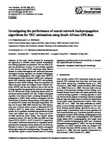
select an appropriate training algorithm for the situation of their work. 2. EXPERIMENT METHOD The experiments were created by used the algorithms GD, GDM, RP, LM for train each neural networks. These algorithms are implemented in a commercial software [3]. The logical functions, or (OR), exclusive or (XOR),3 bit parity (3B) and 5 bit counting (5B) are the training data. The definitions of the logical functions have defined and been used in [2]. For our conveniences, they are reviewed here. The OR training data are the pairs of 2 element input vector and 1 element output vector. The relationship of the input and output is as the original logical function or. For the XOR training data are the pairs of 2 element input vector and 1 element output vector, but the original logical function exclusive or is the relationship of its input and output. In the 3B problem, the network is trained to give the output 1 when then the input vector have the odd number of 1’s. The 5B problem is counting the number of 1s in the input vector. Therefore, the number of network output is 6. When a 5 bit input vector presents the trained network, only the output which the order is corresponding to the number of 1s in the input vector becomes 1. All experiments were performed 30 times for 30 different sets of initial random from uniform distribution weight between -0.3 and 0.3. The algorithms for training neural network were terminated when output mean square error (MSE) reaches 0.001 or when the iteration number are more than 60,000 iterations. For all nodes, their activation functions are the hyperbolic tangent sigmoid transfer function (Tan - Sigmoid) [3]. The architectures of networks are denoted as (a, b, c) and (a, b, c, d) for 3 layers and 4 layers respectively. The, b, c, and d are the number of nodes in each layer of the network. The Figure 1 shows examples of the feedforward networks corresponding to our notation. In the experiments, the networks with different architectures are trained with input-output pairs of logical functions as the following,

The performance comparisons of backpropagation algorithm’s family on a set of logical functions

115

3. EXPERMENT RESULTS

Fig.1: Examples of Network Architectures

¥ the OR problem, the networks are (2,2,1), (2,2,2,1), (2,4,4,1), ¥ the Exclusive-OR problem, the networks are (2,2,1), (2,2,2,1), (2,4,4,1) ¥ the 3-bit parity problem, the networks are (3,3,1),(3,3,3,1),(3,6,6,1), ¥ the 5-bit counting problem, the networks are (5,12,6), (5,5,12,6), (5,12,24,6). In this paper, we also defined a performance index, a ratio of the output squared error sum to the input squared error sum (OSISE), aiming to show the generalization properties of the trained networks. The OSISE can be expressed as in the Equation (1). Ratio of Output Squared Error Sum to Input Squared Error Sum

OSISE =

X

Eo2 /

all

X

Ei2

(1)

all

Output Error Vector [Eo1 . . . Eok ] = [d1 . . . dm ] − [y1 . . . ym ] Input Error Vector [Ei1 . . . Eik ] = [p1 . . . pk ] the input, perturbation, perturbed input and output vectors [x1 . . . xk ] is the input vectoe, [p1 . . . pk ] is the unif orm random perturbation vector, [x1 + p1 . . . xk + pk ] is the pertubed input vector, applying to the evaluated network, [d1 . . . dm ] is the desired output vector, [y1 . . . ym ] is the network output vector. k and m ={1,2,3,.........}

To calculate the OSISE, the all input patterns are added by uniform random perturbation vectors, [p1 . . . pk ] with three certain ranges ±0.01, ±0.1 and ±0.2 . The perturbed input vectors [x1 +p1 . . . xk +pk ] then are applied to the trained forward neural networks to calculate the output. The differences of training vectors and perturbed input-output vectors are the errors. The elements of each error vector are squared and added together. The ratio of the total sum of output squared error to the total sum of input squared error is the OSISE.

The experiment results are shown in Table 1-4. In the tables, there are 6 major columns. The first column is the name of experiment corresponding its setting up. There are 3 parts of the name that the first, the second, and the third mean the training algorithm, the logical function data, and the network architecture. For an example, GDM OR (2,4,4,1) means that the Gradient Descent with Momentum algorithm and the logical function OR are used for training the network having the architecture (2,4,4,1) as in Figure 1(b). The second column is the percentage of successes in training, out of 30 trainings. The third column is the average number of iterations. Only the iteration numbers of the success training are used in the average calculation. The forth column is the standard deviation of the iteration numbers. The fifth column, consisting of 3 sub columns, is the OSISE ratio. The OSISE ratios in each sub column are calculated as defined in the section II starting from generating the input perturbation vector [p1 . . . pk ]. The elements p’s are random having a range over the uniform distribution. The ranges of random perturbation are ±0.01, ±0.1 and ±0.2 for the sub column 1, 2, and 3 respectively. The last column is the number of nodes of the networks. From the Tables 1-4, the percentage of successes in training, the average of iteration numbers and the standard deviation of iteration numbers from the training successes seems to relate to the kind of the logical functions for the GD, GDM and RP algorithms. Only the LM algorithm has the 100% of success training for all kind of logic functions. However, based on the kind of the logical function training data, we do not make general conclusions for GD, GDM and RP on the percentage of training successes. Table 1: Experiment results using the function OR as the training data.

116


Table 2: Experiment results using the function Exclusive OR as the training data.

Table 3: Experiment results using the logical function 3 Bit Parity as the training data.

Fig.3: The relation between the average number of iterations and the number of nodes.

Table 4: Experiment results using the logical function 5 Bit counting as the training data.

Fig.4: The relation between the standard deviation of iterations and the number of nodes.

Fig.2: The relation between the number of nodes and the percentage of successes.

There is another view point. Figure 2 showing a relation between the number of network nodes (column 6) and the percentage of successes (column 1) from Tables 1–4. Once the number of nodes increases, generally the percentage of training successes goes down for the GD, GDM and RP algorithms. The LM algorithm shows the superior performance over the other for having training successes 100%. This means the LM algorithm converges every time of 30 repeated experiments. To evaluate the training speed of each algorithm, the column 3 and 4 of Tables 1–4 are considered. Figure 3 shows the relation between average number of iterations of converged experiments and the number of network nodes. Figure 4 shows the relation between the standard deviation of iteration numbers and the node number of network. The trends of the average and the standard deviation are almost the same. From Figure 3, once the node number more than 20 the GD and GDM take very long to reach the termination. In Figure 4, the standard deviation values of GD and GDM are also very high. This means if one is using GD and GDM for training a network having more than 20 nodes, he cannot expect the convergence time.

The performance comparisons of backpropagation algorithm’s family on a set of logical functions

117

Fig.5: the relation between the OSISE and the training algorithms For the RP and LM in Figure 3, these two algorithms demonstrate on the convergence speed very well. In Figure 4, their standard deviation values are very much smaller comparing to the GD and GDM. Therefore the convergence times of RP and LM are much more predictable. Their convergence times also seem to be independent to number of nodes. They do not increase when the number of node increases. Figure 5 shows the relation between OSISE and the 4 training algorithms. The data to plot these graphs are Tables 1–4. The names of experiments are on the horizontal axis and the OSISE value is the vertical axis. There are 3 vertical bars for each experiment. Each bar represents the OSISE of the input perturbation range ±0.01, ±0.10, and ±0.20. As aforementioned the RP and LM perform very well for the convergence speed, however Figure 5 directly shows the drawback of the fast convergence. The RP and LM have very poor OSISE (too high) comparing to the GD and GDM. The OSISE values of GD and GDM are very small. They are not high enough to appear on the graphs. From this view point, we may roughly classify the training algorithms into 2 groups. The first group, GD and GDM, has slow training speed, low convergence percentage when the number of nodes is large, and low OSISE. The second group, RP and LM, has fast training speed, high convergence percentage for all numbers of nodes, but high OSISE. Surprisingly, the OSISE is very high for the small perturbation with the ±0.01 uniform distribution

range, when the network are trained by using the RP in the experiment RP 3B (3,3,31) in Figure5(c), and in all of the experiments using RP in Figure 5(d). These plots suggest us to have a special care to the input of the system. The RP-training and LM-training system may be sensitive very much to input noise. The signal to noise ratio (SNN) [4] does not need to be low to corrupt the outputs. With a high SNN on the input signal, the output of the networks may be damaged greater than the one with a low SNN. This is an uncommon situation. Usually, the small OSISE is expected when the range of uniform perturbation is small. The large OSISE should be produced from the large uniform perturbation rage. In general, the order of convergence speed agrees with many literatures, e.g. in [1, 2, 5, 6, 7]. The unexpected relation between OSISE and input perturbation range seems very hard to understand. Our experiments here are not enough to provide any explanations to the unexpected relation. This is a topic that calls for further study. The error analysis for multilayer network has not well developed, but only for the single layer network Adaline in [8, 9] is well developed, and practically defined. 4. CONCLUSIONS The GD and GDM algorithms have a good generalization [9] producing the small OSISE. However, they suffer from their convergence ability. The percent-

118


age decreases when the number of nodes is increases. Their training speeds are very poor and hardly to predict because the average and standard deviation of iteration numbers are so large. The RP also suffer from the convergence ability. The percentage of successes in training is lower when the number of nodes increases. In the experiments, when the RP is able to converge, it’s done with a short time producing a low average and a low standard deviation of the iteration numbers. Its convergence iteration number is predictable. The seriously drawback of RP is having the highest OSISE for the small input perturbation. The LM has the superior convergence ability. All LM experiments converge with a small average and standard deviation of iteration numbers. Therefore the convergence iteration number is predictable. The LM suffer from the high OSISE as same as the RP. One has to care the inputs for the LM and RP trained network seriously. A little input noise can corrupt the network output. The LM has the superior convergence ability. All LM experiments converge with a small average and standard deviation of iteration numbers. Therefore the convergence iteration number is predictable. The LM suffer from the high OSISE as same as the RP. One has to care the inputs for the LM and RP trained network seriously. A little input noise can corrupt the network output. The slow training algorithms such as GD and GDM may be considered to use when an application requires the generalization property of the network to achieve accuracy. This paper provides us the general trends of their behaviors. References [1]

[2]

[3] [4]

[5]

Fahlman, S. E., “Fast learning variations on back-propagation: An empirical study,” Proceedings of the 1988 Connectionist Models Summer School (Pittsburgh, 1988), D. Touretzky, D. Hinton, and T. Sejnowski, eds., pp. 38-51. Morgan Kaufmann, San Mateo, California, 1989. S. C. Ng and S. H. Leung, “On solving the local minima problem of adaptive learning by using deterministic weight evolution algorithm,” Evolutionary Computation, 2001. Proceedings of the 2001 Congress on Volume 1, 27-30 May 2001 Page(s):251 - 255 vol. 1 MATLAB, Version 7.0.4.365 (14), Servic Pack 2, Jan 29, 205., Mathworks Inc., US B. P. Lathi, Modern Digital and Analog Communication Systems, Oxford University Press, USA; 3 edition, March 26, 1998 Riedmiller, M.; Braun, H., “A direct adaptive method for faster backpropagation learning: the RPROP algorithm,” Neural Networks, 1993., IEEE International Conference on, Vol., Issue., 1993, Pages:586-591 vol.1

[6]

[7]

[8]

[9]

Hagan, M.T.; Menhaj, M.B., “Training feedforward networks with the Marquardt algorithm,” Neural Networks, IEEE Transactions on, Vol.5, Iss.6, Nov 1994, Pages:989-993 Meng-Hock Fun; Hagan M.T., “LevenbergMarquardt training for modular networks,” Neural Networks, 1996., IEEE International Conference on, Vol.1, Iss., 3-6 Jun 1996, Pages:468-473 Bernard Widrow and S. D. Stearns, Adaptive Signal Processing, Englewood Cliffs, NJ, Prentice-Hall, 1985. Widrow, B.; Lehr, M.A., “30 years of adaptive neural networks: perceptron, Madaline, and backpropagation,” Proceedings of the IEEE, Volume 78, Issue 9, Sept. 1990 Page(s):1415 - 1442

Akaraphunt Vongkunghae received the B.Eng. degree in electrical engineering from Chiang Mai University, Chiang Mai, Thailand, in 1992 and the M.S. degree in electrical engineering from Vanderbilt University, Nashville, TN, in 1998. He received the Ph.D. degree in electrical engineering at the University of Idaho, Moscow, US, in Dec 2004. Currently he is a lecture at Naresuan University, Thailand. His interested researches currently are in global optimization and machine learning.

Anuchit Chumtong received the B.Eng. degree in computer engineering from Naresuan University, Phitsanulok, Thailand, in 2005. He is currently pursuing M.S. degree in electrical engineering at Naresuan University, Phitsanulok, Thailand. His expertise is in microcontroller’s applications. He was the chair of robotics club when he was undergraduate student.