Theory of constraints and linear programming: a reexamination
Jaydeep Balakrishnan Operations Management Area Faculty of Management University of Calgary Calgary Alberta T2N 1N4 Canada Ph: (403) 220 7844 Fax : (403) 284 7902 Email:
[email protected]
Chun Hung Cheng Department of Systems Engineering and Engineering Management The Chinese University of Hong Kong Shatin Hong Kong PRC Email:
[email protected]
Published in the International Journal of Production Research, 38, 6, 2000, 1459-1463.
Abstract In a previous paper in this journal, Luebbe and Finch (1992) compared the Theory of Constraints (TOC) and Linear Programming (LP) using the five-step improvement process in TOC. This paper clarifies some of their results. Specifically, by modifying their example we show that some of their conclusions are not generalizable. Further it is shown using LP is preferable to the $ return/constraint unit method in helping increase throughput and the reasons for this are discussed. Thus LP is a useful tool in the TOC analysis.
Theory of constraints and linear programming: a reexamination
1. Introduction In a previous article in this journal, Luebbe and Finch (1992) compare the Theory of Constraints (TOC) and Linear Programming (LP). They point out that while TOC is a philosophy that may use many techniques, LP is a specific optimization technique. In that article they compare the use of the $ return/constraint unit analysis in TOC and LP using the five step improvement process in TOC. In their examples LP and the $ return/constraint unit analysis give identical results. One important conclusion from this comparison is that level of detail provided by the $ return/constraint unit analysis is more detailed and provides a more sophisticated analysis than LP shadow prices in analyzing changes in processing times and products. This paper shows that these are not conclusions that can be generalized. Using the $ return/constraint unit analysis may result in sub-optimal results when the scenarios that they have used in the article are modified slightly. In addition the reasons for this deficiency in the $ return/constraint unit analysis are discussed. As a result we demonstrate why LP is preferable to the $ return/constraint unit analysis in the TOC improvement process.
2. Analysis of the Luebbe and Finch example In Steps 1 through 3 of the TOC analysis, Luebbe and Finch consider an example with two products, P and Q. In Step 4, this problem is modified by considering an additional export market where the contribution margin is reduced by $9 for P and $10 for Q. The export demands are 50 and 25 units for P and Q respectively. As a result, two additional
1
variables Px and Qx are introduced, where ‘x’ denotes the export market. This gives rise to the following formulation
Maximize z = 45P + 60Q + 36Px + 50Qx Subject to 15P + 10 Q + 15Px + 10Qx 2400 15P + 30 Q + 15Px + 30Qx 2400 15P + 5 Q + 15Px + 5Qx 2400 10P + 5 Q + 10Px + 5Qx 2400 P 100 Q 50 Px 50 Qx 25
(Resource A) (Resource B) (Resource C) (Resource D) (Market for P) (Market for Q) (Export Market for P) (Export Market for Q)
All variables non-negative.
Since Px is identical to P and Qx is identical to Q physically, the processing times for the original and export products are identical.
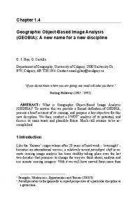
Insert Figure 1 about here
Two scenarios are considered. Scenario 1 is the formulation shown above. In Scenario 2, the processing times on resource B are modified. Figure 1 shows Scenario 1 in the Excel spreadsheet format. Column L gives the utilization of the different resources given the full market potential of the four products. Since row 18 has the highest utilization of 187.5%, resource B is the system constraint and the $ return/constraint unit of B for each product determines the production priority.
2
Row 12 gives the $ return/constraint unit of B. Based on this, the order of priority for production would be P, Px, Q and Qx and the solution as given by the $ return/constraint unit of B analysis is P = 100, Px = 50, Q = 5 and Qx = 0 with a profit of $6600. LP (Excel Solver) gives the same result.
Now assume that the processing times on Resource A (row 31) are changed. P (and P x) now requires 16 minutes and Q (and Qx ) requires 11 minutes. This will have no effect on the $ return/constraint analysis which will still be based on resource B, as although resource A will now have a utilization of 134.4%, resource B with 187.5% remains the system constraint. However the previous solution of P = 100, Px = 50, Q = 5 and Qx = 0 is infeasible as resource A would have a utilization of over 100% with the increased process times. In order to obtain a feasible solution, production of Q, the lowest $ return/constraint unit of B item being produced, is reduced to bring the utilization down to 100%. This will result in P = 100, Px = 50, Q = 0 and Qx = 0 and a a profit of $6300. The utilization of the different resources is shown in Figure 2.
Insert Figure 2 about here
Using the LP Solver however, a higher profit solution of P = 100, Px = 44.8, Q = 7.6 and Qx = 0 with a profit of $6569 is obtained.
3
The sub-optimality of the $ return/constraint unit method can be analyzed by examining Figure 2. Note that though the production decisions were made on the basis of resource B, it is resource A that reaches 100% utilization first. This indicates the inappropriateness of the $ return/constraint unit analysis in a situation where an apparently non-system constraint impacts on the $ return/constraint unit analysis. This aspect will be discussed further in the next section.
Further assume that additional units of resource B are available at some cost. Based on the utilization in Figure 2 (from the $ return/constraint unit of B analysis) there is no value in acquiring additional units of B as it is not utilized fully at present. But an examination of the LP sensitivity analysis report will reveal that both resources A and B are utilized fully given the LP optimal solution. Thus the shadow price of resource B is positive ($1.8). Therefore depending on the cost, additional units of resource B might be beneficial. The shadow price indicates the additional money (or throughput in TOC) that can be generated from an additional unit of a resource. Further, given the $0.6 shadow price of A, LP indicates that the throughput resulting from an additional unit of resource B is higher than that for A. So the shadow price is useful in prioritizing resources for throughput increase. Thus the LP shadow price is more reliable and useful than the $ return/constraint unit analysis in valuing resources. Also note that the under-utilization of resource B results in the sub-optimal profit of the $ return/constraint unit analysis.
The result is similar in Scenario 2 where Luebbe and Finch reduce processing times on Resource B (Table 4 in Luebbe and Finch), thus making Resource A the system
4
constraint with 125% utilization. Based on the $ return/constraint unit analysis, the order of priority for production is Q, P, Qx and Px. The $ return/constraint unit analysis and LP solution is P = 100, Px = 10, Q = 50 and Qx = 25. Again, if the processing times on resource B are changed such that P (and Px) requires 9.5 minutes and Q (and Qx ) requires 19 minutes, there is no change in the $ return/constraint unit analysis as resource A remains the system constraint. However, the previous solution of P = 100, P x = 10, Q = 50 and Qx = 25 is infeasible for the new processing times as resource B will have a utilization of 103%. Thus based on the $ return/constraint unit analysis, production of Px, the item with the lowest $ return/constraint unit of A, would be reduced, which would result in a product mix of P = 100, Px = 2.3, Q = 50 and Qx = 25 with a profit of $8845. Again, this is sub-optimal. The optimal solution is P = 100, Px = 13.7, Q = 50 and Qx = 19.5 with a higher profit of $8966.
Similarly, it can be shown easily from the spreadsheet that with the feasible $ return/constraint unit analysis solution of P = 100, Px = 2.3, Q = 50 and Qx = 25, resource A would be under-utilized causing the sub-optimal profit of $8845. In addition, based on the $ return/constraint unit analysis, one would conclude that there is no value in acquiring additional units of resource A. The LP sensitivity analysis report will show otherwise.
3 Analysis of the results As demonstrated in the previous section, the $ return/constraint unit cannot be generalized. It works well when only one resource is overloaded given full market
5
potential. In this case, the problem reduces to one with a single constraint as the nonsystem constraints are redundant and the $ return/constraint unit will give the optimal solution. This is true in the original two-product problem solved in Luebbe and Finch. In the four-product case, it is seen that in Scenario 1, resources A, B and C are overloaded (Figure 1). In Scenario 2 resources A and C are overloaded. In such situations the $ return/constraint unit analysis examines only the system constraint and ignores the other overloaded constraints. As a result, in our modified problems, an apparently non-system constraint reached 100% utilization first preventing full exploitation of the system constraint.
This gives rise to an important question – what is the system constraint? For example in Scenario 1, is it the one that is the most overloaded given the market potential (resource B)? Or is it Resource A, which is the first resource to reach 100% utilization when implementing the $ return/constraint unit analysis? TOC does not address this conflict. This paper shows that it is not easy to identify the system constraint a-priori in multiple constraint (given market potential) situations. Thus the $ return/constraint unit analysis being dependant on this a-priori identification and by examining only one constraint does not guarantee full exploitation of the system. LP being an optimization technique does exploit the system fully.
The $ return/constraint unit analysis is a heuristic that examines only a few LP corner solutions. It satisfies a higher priority product’s market demand before moving to the lower priority product. This priority is based on the system constraint only. Thus it does
6
not look at beneficial corner points where a lower priority product may be produced without completely satisfying a higher priority product’s market demand as was the case in Scenarios 1 and 2. For problems involving more products and resources, the $ return/constraint unit method will only examine a minute proportion of the possible corner point solutions. Using LP would be a preferable method of arriving at optimal solutions and analyzing changes in the processing times and products. Thus LP will help achieve the maximum throughput most efficiently.
Finally, as was discussed in the previous section, a disadvantage of not obtaining the optimal solution is that the value of different resources may be evaluated incorrectly. In both Scenarios 1 and 2, the $ return/constraint unit analysis would assume that additional amounts of some of the resources would be of no value, whereas in reality they do have value. LP shadow prices can correctly determine the relative value of additional resources. This aspect is very important as the focus of TOC is increasing throughput. Since adding resources can increase throughput it is important to have a tool such as LP that help achieve the increased throughput correctly and efficiently.
4. Conclusion Using LP in the various stages of the five-step TOC analysis is preferable to the $ return/constraint unit analysis in the case of multiple constraint situations. LP can be viewed as an important tool in ensuring that the principles of TOC are applied correctly and increasing throughput efficiently. Since most spreadsheets now have LP solvers included, incorporating LP should not pose a problem for users of TOC. The $
7
return/constraint is useful in explaining the concept of constrained optimization but as a tool in the five-step TOC process it is deficient.
Acknowledgement The authors wish to recognize the financial support of the Natural Sciences and Engineering Research Council of Canada (NSERC) for this research.
References: 1.
Luebbe R. and Finch B., 1992, Theory of constraints and linear programming. International Journal of Production Research, 30, 1471-1478.
8
C 3 4 5 6 7 8 9 10 11 12 13 14 15 16 17 18 19 20 21 22 23 24 25 26 27 28 29 30 31 32 33 34 35
D
E
F
G
H
Decision variables
I
J
K
L
Total Profit = 45P + 60Q + 36P(x) + 50Q(x)
RESULTS P
Q
P(x)
Q(x)
Units produced Contribution Margin Profit
100 45 4500
50 60 3000
50 36 1800
25 50 1250
$ Return/Const. B
3
2
2.4
1.67
10550
TOTAL RESOURCES USED AND MARKET SATISFIED
Resource A Resource B Resource C Resource D Market for P (units) Market for Q (units) Market for P(x) (units) Market for Q(x) (units)
1500 1500 1500 1000 100
500 1500 250 250
750 750 750 500
250 750 125 125
50 50 25
RESOURCES REQUIRED PER UNIT OF OUTPUT P Q Resource A 15 10 Resource B 15 30 Resource C 15 5 Resource D 10 5
P1 15 15 15 10
Total Used 3000 4500 2625 1875 100 50 50 25
Available