treat linear real-time specifications that are given as deterministic timed au- tomata (DTA). .... attached to the transitions. s0 start. {a} r0 s1. {a} r1 s2. {a b} r2 s3. {0} r3 s5. {c} r5 s4. {c} r4. 1. 0.5 ...... Complete set of linear inequalities. Changing all ...
Time-Bounded Verification of CTMCs Against Real-Time Specifications ? Taolue Chen, Marco Diciolla, Marta Kwiatkowska, and Alexandru Mereacre Department of Computer Science, Oxford University, Wolfson Building, Parks Road, Oxford, OX1 3QD, United Kingdom
Abstract. In this paper we study time-bounded verification of a finite continuous-time Markov chain (CTMC) C against a real-time specification, provided either as a metric temporal logic (MTL) property ϕ, or as a timed automaton (TA) A. The key question is: what is the probability of the set of timed paths of C that satisfy ϕ (or are accepted by A) over a time interval of fixed, bounded length? We provide approximation algorithms to solve these problems. We first derive a bound N such that timed paths of C with at most N discrete jumps are sufficient to approximate the desired probability up to ε. Then, for each discrete path σ of length at most N , we generate timed constraints over variables determining the residence time of each state along σ, depending on the real-time specification under consideration. The probability of the set of timed paths, determined by the discrete path and the associated timed constraints, can thus be formulated as a multidimensional integral. Summing up all such probabilities yields the result. For MTL, we consider both the continuous and the pointwise semantics. The approximation algorithms differ mainly in constraints generation for the two types of specifications.
1
Introduction
Verification of continuous-time Markov chains (CTMCs) has received much attention in recent years [7]. Thanks to considerable improvements of algorithms, (symbolic) data structures and abstraction techniques, CTMC model checking has emerged as a valuable analysis technique. Aided by powerful software tools, it has been adopted by researchers from, e.g., systems biology, queuing networks and dependability. The focus of CTMC model checking has primarily been on checking stochastic versions of the branching-time temporal logic CTL, such as CSL [6]. The verification of LTL properties reduces to applying well-known algorithms [31,16] to embedded discrete-time Markov chains (DTMCs). Linear-time properties equipped with timing constraints have only recently been considered. In particular, [14,15] treat linear real-time specifications that are given as deterministic timed automata (DTA). These include properties of the form, “what is the probability to ?
This work is supported by the ERC Advanced Grant VERIWARE.
reach a given target state within the deadline, while avoiding unsafe states and not staying too long in any of the dangerous states on the way?”. Such properties can neither be expressed in CSL nor in its dialects [5,17]. Model checking DTA properties can be done by a reduction to computing the reachability probability in a piecewise deterministic Markov process, based on the product construction between the CTMC and DTA [15,9]. It remains a challenge to tackle more general real-time specifications like Metric Temporal Logics ([3,22], MTL), or nondeterministic Timed Automata (TA, [1]). The main difficulty lies in the fact that one cannot easily define a stochastic process out of the CTMC and the MTL formula (or TA), due to the inherent nondeterminism arising from these specifications. The obstacle is somehow fundamental, as it is known that deterministic TA are lacking expressiveness compared to their nondeterministic variants or MTL. Recently, we have seen increasing emphasis on timed-bounded verification [25]. Here, “time-bounded” means restricting the modeling and verification efforts to some bounded interval of time, which itself can be taken as a parameter. In verification, queries are phrased over time intervals of fixed, bounded duration. Note that, differently from bounded model checking, which restricts the total number of allowable events (called discrete jumps in this paper), timebounded verification restricts the total duration under consideration, but not the number of events, which can still be unboundedly large owing to the density of time.1 Instances of time-bounded verification have been considered in the context of stochastic and/or real-time systems [28,8,21,18] and recently studied systematically [25,20]; see [27] for an introduction, where it is argued that the restriction on total duration is very natural for real-time systems. Inspired by this recent progress, we study the time-bounded verification problem of a CTMC C, against a real-time specification provided as either an MTL formula ϕ, or as a TA A. The key question is: what is the probability of the set of timed paths of C that satisfy ϕ (or are accepted by A) over a fixed time interval [0, T ] where T ∈ R>0 ? We provide approximation algorithms to solve these problems. Given any ε > 0 a priori, we first derive a bound N such that it is sufficient only to consider timed paths of C with at most N discrete jumps to approximate the desired probability up to ε. Then, for each discrete path σ of C of length at most N , we generate a family of linear constraints, S, over variables determining the residence time of each state in σ. The discrete path σ, together with the associated timing constraints S, determinates a set of timed paths of C, each of which satisfies ϕ (or is accepted by A). The probability of this set of timed paths can be formulated as a multidimensional integral, which can be calculated by Laplace transforms, together with an application of the inclusion-exclusion principle. Summing up all such probabilities yields the desired result. Notice that, in the current paper, we consider both the continuous and the pointwise semantics of MTL (see, e.g. [12]). The approximation algorithms differ mainly in constraints generation for different types of specifications. 1
Readers should notice that we later bound the number of discrete jumps as an approximation technique. This owes to the definition of CTMCs and is irrelevant to the original definition of time-bounded verification.
2
The family of linear constraints are desirable, since we can apply the efficient algorithm for computing the volumes of convex polyhedra [23]. For MTL under the pointwise semantics and TA specifications, constraint generation is relatively easy, while for MTL under the continuous semantics it is more involved. To this end, we first derive constraints in terms of first-order theory of (R, +, −, 0, 1, ≤), then the Fourier-Motzkin elimination procedure [29, pp.155-156] is applied to obtain desired linear constraints. We believe these results are of independent interest, as they have potential usage in areas like runtime verification. The approach we take in this paper is quite different from the existing results in literature. Known results can only deal with simpler real-time properties, or are based on deterministic property specifications (e.g. DTA). Our technique is based on path exploration of CTMCs, together with a novel analytic methodology to reduce computing probabilities to multi-dimensional integral over convex polyhedra. To the best of our knowledge, this is the first work addressing verification of CTMCs against MTL formulas or timed automata. We remark that since the probabilities in question are reals in general, approximation algorithms are the best we can expect. Related work. Model checking CTMCs against linear real-time specifications has received scant attention so far. To our knowledge, this issue has only been (partially) addressed in [14,5,17]. Baier et al. [5] define the logic asCSL where path properties are characterized by (time-bounded) regular expressions over actions and state formulas. The truth value of path formulas depends not only on the available actions in a given time interval, but also on the validity of certain state formulas in intermediate states. asCSL is strictly more expressive than CSL [5]. Model checking asCSL is performed by representing the regular expressions as finite-state automata, followed by computing time-bounded reachability probabilities in the product of CTMC C and this automaton. In CSLTA [17], time constraints of until modalities are specified by a single-clock DTA; the resulting logic is at least as expressive as asCSL [17]. The combined behavior of C and the DTA A is interpreted as a Markov renewal process, and model checking CSLTA is reduced to computing the reachability probabilities in a DTMC whose transition probabilities are given by subordinate CTMCs.
2 2.1
Preliminaries Continuous-time Markov chains
Given a set H, let Pr: F(H) → [0, 1] be a probability measure on the measurable space (H, F(H)), where F(H) is a σ-algebra over H. Let Distr (H) denote the set of probability measures on this measurable space. Definition 1 (CTMC). A (labeled) continuous-time Markov chain (CTMC) is a tuple C = (S, AP, L, α, P, E) where – S is a finite set of states; 3
– – – – –
AP is a finite set of atomic propositions; L : S → 2AP is the labeling function; α ∈ Distr (S) is the initial distribution; P : S × S → [0, 1] is a stochastic matrix; and E : S → R≥0 is the exit rate function.
Example 1. An example CTMC is illustrated in Fig. 1, where AP = {a, b, c} and s0 is the initial state, i.e., α(s0 ) = 1 and α(s0 ) = 0 for any s 6= s0 . The exit rates are indicated at the states, whereas the transition probabilities are attached to the transitions. {∅} s3
0.2
{a} start
1
s0 r0
s1 0.5
r3
0.7
{a}
{a b} 0.5
{c} 0.8
s5
1
r5
s2
r1
r2
0.3
{c} s4
1
r4
Fig. 1. An example CTMC In a CTMC C, state residence times are exponentially distributed. More precisely, the residence time X of a state s ∈ S is a random variable governed by a nonnegative exponential distribution with parameter E(s) (written as X ∼ Exp(E(s))). Hence, the probability to exit state s in t time units (t.u. for short) is Rt given by 0 E(s) · e−E(s)τ dτ . Furthermore, the probability to take the transition Rt from s to s0 in t t.u. equals P(s, s0 ) · 0 E(s) · e−E(s)τ dτ . A state s is absorbing if P(s, s0 ) = 1. The embedded discrete-time Markov chain (DTMC) of CTMC C is obtained by deleting the exit rate function E, i.e., emb(C) = (S, AP, L, α, P). Definition 2. Given a CTMC C = (S, AP, L, α, P, E), we define the following notions. – A (finite) discrete path σ = s0 → s1 → s2 → . . . is a (finite) sequence of states; we define σi to be the state si , and σ i to be the prefix of length i of σ. x0 x1 x2 – A (finite) timed path ρ = s0 −→ s1 −→ s2 −→ . . ., where xi ∈ R>0 for each i ≥ 0, is a sequence starting in state s0 ; we define |ρ| to be the length of a finite timed path ρ; ρ[n] := sn is the n-th state of ρ and ρhni := xn is the time spent in state sn ; let ρ@t be the state occupied in ρ at time t ∈ R≥0 , n P i.e. ρ@t := ρ[n], where n is the smallest index such that ρhii ≥ t. i=0
– Given a finite discrete path σ = s0 → s1 → · · · → sn−1 of length n and x0 , . . . , xn−1 ∈ R>0 , define σ[x0 , . . . , xn−1 ] to be the finite timed path ρ such that ρ[i] := si and ρhii := xi for each 0 ≤ i < n. – Let Γ be the set of n-tuples (x0 , . . . , xn−1 ) ∈ Rn>0 , then σ[Γ ] = {σ[x0 , . . . , xn−1 ] | (x0 , . . . , xn−1 ) ∈ Γ }. 4
– Given a finite (resp. infinite) discrete path σ and a finite (resp. infinite) timed path ρ, we say σ is the skeleton of ρ if for each i ≥ 0, σi = ρ[i]. We write S(ρ) for the skeleton of ρ, and for a set of (finite or infinite) timed paths Ξ, we write S(Ξ) = {S(ρ) | ρ ∈ Ξ}. – Given a finite discrete path σ, we define Cd (σ) = {σσ 0 | σ 0 is an infinite discrete path} to be the set of all infinite discrete paths with the same common prefix σ. Intuitively, a timed path ρ suggests that the CTMC C starts in state s0 and stays in this state for x0 t.u., and then jumps to state s1 , staying there for x1 3 t.u., and then jumps to s2 and so on. An example timed path is ρ = s0 −→ 2 1.5 3.4 s1 −→ s0 −→ s1 −→ s2 . . . with ρ[2] = s0 and ρ@4 = ρ[1] = s1 . Let Paths C denote the set of infinite timed paths in the CTMC C, and Paths C (s) the set of infinite timed paths in C that start in s. Given a time bound T ∈ R≥0 and N ∈ N ∪ {∞}, we define ( ) k X C C ρhii ≥ T , Paths T, 0 for 0 ≤ i < k and I0 , . . . , Ik−1 be nonempty intervals in R≥0 . Let C(s0 , I0 , . . . , Ik−1 , sk ) denote the cylinder set consisting of all ρ ∈ Paths(s0 ) such that, ρ[i] = si (i ≤ k), and ρhii ∈ Ii (i < k). F(Paths(s0 )) is the smallest σ-algebra on Paths(s0 ) which contains all sets C(s0 , I0 , . . . , Ik−1 , sk ) for all state sequences (s0 , . . . , sk ) ∈ S k+1 with P(si , si+1 ) > 0 for (0 ≤ i < k) and I0 , . . . , Ik−1 range over all sequences of nonempty intervals in R≥0 . The probability measure PrC on F(Paths(s0 )) is the unique measure defined by induction on k by PrC (C(s0 )) = α(s0 ) and for k > 0: PrC (C(s0 , I0 , . . . , Ik−1 , sk )) = PrC (C(s0 , I0 , . . . , Ik−2 , sk−1 )) Z × P(sk−1 , sk )E(sk−1 ) · e−E(sk−1 )τ dτ . Ik−1
In general, computing the probability of a cylinder set with k intervals I0 . . . Ik−1 (i.e. k discrete jumps) reduces to calculating a k-dimensional integral over I0 . . . Ik−1 . 5
Example 2. Consider, the CTMC C in Figure 1 and the simple cylinder set C(s0 , I0 , s1 , I1 , s0 ) where I0 , I1 ∈ R≥0 . The probability of C in C can be calculated as: P rC (C(s0 , I0 , s1 , I1 , s2 )) = P(s0 , s1 )P(s1 , s0 )E(s0 )E(s1 ) Z Z × e−E(s0 )τ1 −E(s1 )τ2 dτ2 dτ1 I0
2.2
(1)
I1
Metric Temporal Logic
Definition 3 (Syntax of MTL). Let AP be an arbitrary nonempty, finite set of atomic propositions. Let I = [a, b] be an interval such that a, b ∈ N ∪ {∞}. The Metric Temporal Logic is inductively defined as: ϕ ::= p | ¬ϕ | ϕ1 ∧ ϕ2 | ϕ1 UI ϕ2 , where p ∈ AP and ϕ1 , ϕ2 are MTL formulas. We introduce two time-bounded semantics for MTL, as follows. Definition 4 (Continuous Semantics). Given an MTL formula ϕ, a time bound T , a timed path ρ and a variable t ∈ R≥0 , the satisfaction relation (ρ, t) |=cT ϕ is inductively defined as follows: (ρ, t) |=cT (ρ, t) |=cT (ρ, t) |=cT (ρ, t) |=cT
p ¬ϕ1 ϕ1 ∧ ϕ2 ϕ1 UI ϕ2
⇔ p ∈ L(ρ@t) ∧ t ≤ T ⇔ (ρ, t) 6|=cT ϕ1 ⇔ (ρ, t) |=cT ϕ1 ∧ (ρ, t) |=cT ϕ2 ⇔ ∃t0 . t ≤ t0 ≤ T s.t. t0 − t ∈ I ∧ (ρ, t0 ) |=cT ϕ2 ∧ ∀t00 . t ≤ t00 < t0 ⇒ (ρ, t00 ) |=cT ϕ1
where p ∈ AP and ϕ1 , ϕ2 are MTL formulas. Definition 5 (Pointwise Semantics). Given an MTL formula ϕ, a time bound T , a timed path ρ and i ∈ N, the satisfaction relation (ρ, i) |=pT ϕ is inductively defined as follows: (ρ, i) |=pT (ρ, i) |=pT (ρ, i) |=pT (ρ, i) |=pT
p ¬ϕ1 ϕ1 ∧ ϕ2 ϕ1 UI ϕ2
Pi ⇔ p ∈ L(ρ[i]) ∧ k=0 ρhki ≤ T ⇔ (ρ, i) 6|=pT ϕ1 ⇔ (ρ, i) |=pT ϕ1 ∧ (ρ, i) |=pT ϕ2 Pi0 ⇔ ∃i0 . i ≤ i0 s.t. k=i ρhki ∈ I ∧ (ρ, i0 ) |=pT ϕ2 ∧ ∀i00 . i ≤ i00 < i0 ⇒ (ρ, i00 ) |=pT ϕ1
where p ∈ AP, ϕ1 , ϕ2 are MTL formulas and i0 , i00 ∈ N. 6
2.3
Timed Automata
Let X = {x1 , . . . , xp } be a set of nonnegative real-valued variables called clocks. An X -valuation is a function η : X → R≥0 assigning to each variable x ∈ X a nonnegative real value η(x). Let V(X ) denote the set of all valuations over X . A clock constraint on X , denoted by g, is a conjunction of expressions of the form x ./ c for x ∈ X , ./ ∈ {, ≥} and c ∈ N. Let B(X ) denote the set of clock constraints over X . An X -valuation η satisfies constraint x ./ c, denoted η |= x ./ c, if and only if η(x) ./ c; it satisfies a conjunction of such expressions if and only if η satisfies all of them. Let 0 denote the valuation that assigns 0 to all clocks. For a subset X ⊆ X , the reset of X, denoted η[X := 0], is the valuation η 0 such that ∀x ∈ X. η 0 (x) := 0 and ∀x ∈ / X. η 0 (x) := η(x). For δ ∈ R≥0 and 00 X -valuation η, η + δ is the X -valuation η such that ∀x ∈ X . η 00 (x) := η(x) + δ, which implies that all clocks proceed at the same speed. Definition 6 (TA). A timed automaton is a tuple A = (Σ, X , Q, q0 , QF , →) where – – – – –
Σ is a finite alphabet; X is a finite set of clocks; Q is a non empty finite set of locations with initial location q0 ∈ Q; QF is a set of final locations; The relation →⊆ Q × Σ × B(X ) × 2X × Q is an edge relation. a,g,X
We refer to q −→ q 0 as an edge, where a ∈ Σ is an input symbol, the guard g is a clock constraint on the clocks of A, X is the set of clocks that must be reset a,g,X and q 0 is the successor location. Intuitively, the edge q −→ q 0 asserts that the 0 TA A can move from location q to location q when the input symbol is a and the guard g holds, while the clocks in X should be reset when entering q 0 . In case no guard is satisfied in a location for a given clock valuation, time can progress. For the sake of simplicity we omit invariants from the definition of TAs. However the results presented here can be easily extended to TAs enhanced with invariants. Definition 7. Given a timed automaton A, we define the following notions. – A discrete path of A is a sequence of states w = q0 → q1 . . . → qn · · · where each qi ∈ Q. a0 ,t0
a1 ,t1
an−1 ,tn−1
– A timed path of A is of the form θ = q0 −→ q1 −→ . . . qn−1 −→ qn · · · such that η0 = 0, and for all i ≥ 0, ai ∈ Σ and it holds ti > 0, ηi + ti |= gi where gi is the guard on the i-th transition, ηi+1 = (ηi + ti )[Xi := 0], where ηi is the clock evaluation when entering qi . We say that θ is accepting if there exists some n ≥ 0 s.t. qn ∈ QF . Definition 8 (Time-bounded Acceptance). Assume a CTMC C = (S, AP, L, s0 , P, E) and a TA A = (2AP , X , Q, q0 , QF , →). A CTMC timed path ρ = 7
t
t
1 0 . . ., is accepted by A if there exists n ∈ N+ and a corresponding s1 −→ s0 −→ TA finite path:
L(s0 ),t0
L(sn−1 ),tn−1
L(s1 ),t1
θ = q0 −→ q1 −→ . . . qn−1 −→ qn , Pn−1 such that qn ∈ QF and i=0 ti ≤ T . We write ρ |=T A to denote that the CTMC timed path ρ is accepted by A. Remark 1. It is possible that a single CTMC timed path corresponds to multiple TA accepting paths due to the nondeterminism of TA.
3
A Bound on the Number of Discrete Jumps
In this section, we give a bound on discrete jumps of paths of CTMCs such that, when verifying an MTL formula or TA, one only needs to consider those paths whose discrete jumps number at most N . The intuition is that, for a given time interval [0, T ], the probability of the set of timed paths which “jump” very frequently is actually very small. Throughout this section we assume a CTMC C = (S, AP, L, α, P, E). For any n ∈ N, we define V n (s, x) : S × R≥0 → [0, 1] as follows: V 0 (s, x)=1 and Z x X V n+1 (s, x) = E(s)e−E(s)τ · P(s, s0 ) · V n (s0 , x − τ )dτ . 0
s0 ∈S
Lemma 1. For all N ∈ N, PrC (Paths CT,≥N (s)) = V N (s, T ). Proof. By induction on N . 1. N = 0: V 0 (s, T ) = 1. This is exactly the probability of all paths {ρ ∈ Paths C (s) | ρh0i ≤ T } that is PrC (Paths CT,≥0 (s)). PrC (Paths CT,≥0 (s)) is the probability to have 0 jumps in the interval of time [0, T ] which is equal to e−E(s)T plus the probability of having more than one jumps in [0, T ] that is 1 − e−E(s)T . Summing up the two probabilities yields 1 as result. 2. Induction step. Z T X V N +1 (s, T ) = E(s)e−E(s)τ · P(s, s0 )V N (s, T − τ )dτ 0
Z
s0 ∈S T
E(s)e−E(s)τ ·
= 0 C
= Pr
X
P(s, s0 )PrC (Paths CT,≥N (s))dτ
s0 ∈S C (Paths T,≥N +1 (s))
t u We then show how to bound V N (s, T ) analytically. ! Given a CTMC C, let ∞ i X (ΛT ) Λ = maxs∈S E(s) and �(T, N ) = e−ΛT · . i! i=N
8
Lemma 2. T
Z
Λe−Λτ · �(T − τ, N )dτ .
�(T, N + 1) = 0
Proof. Z
T
Λe−Λτ · �(T − τ, N )dτ
0 T
Z
Λe−Λτ · e−Λ(T −τ ) · (
= 0
X (Λ(T − τ ))i )dτ i!
i≥N
= e−ΛT = e−ΛT
T
X (Λ(T − τ ))i Λ·( )dτ i! 0 i≥N XZ T (Λ(T − τ ))i )dτ Λ·( i! 0
Z
i≥N
= e−ΛT
X
−
i≥N
= e−ΛT
(Λ(T − τ ))i+1 T |0 (i + 1)!
X (ΛT )i+1 (i + 1)!
i≥N
= e−ΛT
X (ΛT )i (i)!
i≥N +1
= �(T, N + 1). t u Combining Lem. 1 and Lem. 2, we obtain the following Theorem 1. Given a CTMC C, a time bound T and N ∈ N PrC (Paths CT,≥N ) ≤ �(T, N ). Proof. By induction on N . The base case (i.e., N = 0) is straightforward. For N + 1 we have PrC (Paths CT,≥N +1 ) =
Z
T
E(s)e−E(s)τ ·
0
Z
E(s)e−E(s)τ ·
0
Z 0
P(s, s0 ) · PrC (Paths CT −τ,≥N (s0 ))dτ
s0 ∈S T
≤ ≤
X
X
P(s, s0 ) · �(T − τ, N )dτ
s0 ∈S T
Λe−Λτ ·
X
P(s, s0 ) · �(T − τ, N )dτ
s0 ∈S
9
From Lemma 2 we have that Z T X Λe−Λτ · P(s, s0 ) · �(T − τ, N )dτ 0
s0 ∈S
=
X
0
X
T
Λe−Λτ · �(T − τ, N )dτ
P(s, s ) · 0
s0 ∈S
=
Z
P(s, s0 ) · �(T, N + 1)
s0 ∈S
= �(T, N + 1). It follows that PrC (Paths CT,≥N +1 ) ≤ �(T, N + 1), which completes the induction step. t u Proposition 1. Let ε ∈ R>0 and T ∈ R≥0 . For any N ≥ ΛT e2 + ln( 1ε ) we have that �(T, N ) < ε. Proof. We have that �(T, N ) = e
−ΛT
·
∞ X (ΛT )i i!
!
i=N
(ΛT )N ≤ e−ΛT · eΛT · N! � �N ΛT e (ΛT )N ≤ = (N/e)N N � �ln(1/ε) 1 ≤ =ε e t u
.
Remark 2. Readers who are familiar with Poisson distributions will immediately notice that the bound we obtained is actually the probability that there are at least N Poisson arrivals in an interval of time [0, T ], with rate Λ. If the CTMC C is uniform (i.e., each state of C has the same exit rate), then one could obtain the bound in a straightforward way. However, for the general case, this cannot be achieved directly. Moreover, we point out here that, in order to verify an MTL formula ϕ or a TA A, one cannot apply the unformization technique, which is ubiquitous in CTMC model checking.
4
MTL Specifications
In this section we study the problem of model checking CTMCs against MTL properties. Let PrCT (ϕ) := PrC ({ρ ∈ Paths CT | (ρ, 0) |=cT ϕ}) denote the probability that the CTMC C satisfies the MTL formula ϕ, for a given time bound 10
T . Notice that here the definition of PrCT (ϕ) is for the continuous semantics of MTL. We present an algorithm to deal with MTL in pointwise semantics. Instead of computing PrCT (ϕ), we give a procedure to compute PrCT, T ∧ t0 + . . . + tN −2 < T ) ∧
j∈Ji
^
tk > 0 .
0≤k0 |A` · t E Wk b` } defines a convex set. In case that the union `=0 C` is not convex, we use the inclusion-exclusion principle to compute PrC (σ[S]) as follows: C
Pr (σ[S]) =
k X
PrC (σ[C` ]) −
`=0
X
X
PrC (σ[Ci ∧ Cj ]) +
i,j:0≤i