Time Domain Evaluation of Filterless Grid-Connected Multilevel PWM Converter Voltage Quality A. Ruderman (1)
(1)
and B. Reznikov ( 2)
Elmo Motion Control Ltd., General Satellite Corporation
[email protected],
[email protected]
Abstract–Voltage total harmonic distortion and related quadratic criteria are accepted as figures of merit of a multilevel PWM converter voltage quality. The dominating frequency domain voltage quality evaluation approach, in fact, is essentially numerical as it involves infinite double Fourier series expansion with Bessel function coefficients and requires high switching harmonics count. Suggested time domain approach for multilevel PWM converter voltage quality evaluation delivers simple piecewise analytical solutions that clearly reveal the dependence on modulation index for an arbitrary number of voltage levels. The results are applicable to any type of multilevel converters with optimal nearest three space vector PWM allowing for fast comparative evaluation of voltage quality for filterless gridconnected converters with different levels count.
I.
( 2)
INTRODUCTION
Multilevel converters are being progressively used for medium and high voltage / power applications [1, 2] including renewable energy utility interfaces, static power compensators, active power filters, medium voltage drives etc. Passive grid filters typically used to meet the harmonics limits according to IEEE, VEDW, and IEC standards are bulky and may cause parasitic resonance associated problems in mains. Increasing the number of converter voltage levels allows filterless grid connection that is beneficial in terms of system cost, efficiency, power density, and reliability [3]. Most popular multilevel voltage source topologies include diode-clamped (Neutral Point Clamped - NPC - for 3-level), capacitor-clamped (flying capacitor), and cascaded H-bridge topologies [2], and modular multilevel [4]. Recently, Active NPC (ANPC) converter topologies attracted considerable interest [3, 5]. It is actually a merge between diode-clamped (3level NPC) and flying capacitor topologies with level count increase achieved by adding flying capacitor cells. High apparent switching frequency Pulse Width Modulation (PWM) for grid-connected applications has an advantage of generating high quality voltage waveforms free of fundamental frequency harmonics as opposed to fundamental frequency switching (even with selected harmonics elimination). With converter level count increase, individual semiconductor device switching frequency may be significantly reduced for the same apparent switching frequency. For any converter topology, optimal PWM voltage quality is achieved using nearest three space vector type modulation. Converter voltage quality is essentially improved with voltage level count increase [2, 6-8]. The accepted voltage quality evaluation methodology is to analyze voltage Total Harmonic Distortion (THD) in frequency domain. For DC/AC converters, this requires double Fourier
978-1-4244-6392-3/10/$26.00 ©2010 IEEE
infinite series [2, 6, 7]. Such an approach could hardly be considered true analytical. It is rather algorithmic, processor run time consuming (because 30-50 switching harmonics are typically accounted for), and not easy to apply in an everyday engineering practice. In this paper, it is suggested to evaluate converter voltage waveform quality in time domain using ripple voltage Normalized Mean Square (NMS) criterion that may be easily converted into voltage THD. For an arbitrary voltage level, a solution for the ripple voltage NMS is piece-wise analytical and employs elementary functions only that makes suggested approach a preferred choice when a detailed knowledge of PWM voltage harmonic spectrum is not required. This methodology is asymptotic in the sense that the ratio of PWM and fundamental frequencies is assumed infinitely large and, thus, the ripple voltage NMS expressions depend on modulation index only. Alternatively, this approach may be understood as quasi-static in time domain meaning that a fundamental signal is assumed constant on a switching period. For multilevel DC/AC converters, the ripple voltage NMS is obtained by double time integration (averaging) of a normalized ripple voltage square - on a PWM period and on a fundamental one - that is time domain equivalent of the frequency domain double Fourier transform. The solution first found for a single-leg converter is shown to be valid for a three-phase converter with a balanced load as well. Comparison with the frequency domain analysis results demonstrates a real power of the true analytical solution that reveals the way voltage quality depends on modulation index. II. RIPPLE VOLTAGE NMS FOR H-BRIDGE DC PWM For a 2-level H-bridge converter with unipolar PWM, normalized PWM voltage and ripple voltage (that is zero on average) are presented in Fig.1. According to Fig.1,b, the ripple voltage NMS criterion by definition is calculated as
NMS 2DC ( D) = (1 − D) 2 D + (− D) 2 (1 − D) =
(1)
= D(1 − D),
2940
v = V / VDC
vR 1− D
1
0
t /T 0
D
t /T D
1
−D
1
Fig. 1. 2-level H-bridge converter normalized PWM voltage (a) and PWM ripple voltage (b)
v = V / VDC
v = V / VDC
1 0.5 0
Ripple Voltage NMS Criterion for H-Bridge AC PWM
1 t 0.5 0
0.25
t
2-Level 0.2
NMS, p.u.
Fig. 2. 3-level H-bridge converter normalized PWM voltage: a - D=0.25; b – D=0.75
where D - normalized DC voltage command (duty ratio for 2level unipolar PWM). For a 3-level H-bridge converter, normalized nearest level PWM voltages are given in Fig.2 and the NMS is
0.15
0.1
3-Level
D(0.5 − D ), 0 ≤ D < 0.5; NMS3DC ( D ) = (2) ( D − 0.5)(1 − D ), 0.5 ≤ D < 1.
0.05
4-Level 0
Similar to (1), (2), it is possible to obtain the DC PWM NMS for a general case of an arbitrary number of levels L -
i i + 1 − D ; NMS LDC ( D ) = D − − − L 1 L 1 i i +1 ; i = 0,1,..., L − 2. ≤D< L −1 L −1
0
(3)
MAX {NMS LDC ( D )} = 0.25 /( L − 1) 2 .
(4)
Consider sinusoidal normalized voltage command
For PWM frequency much higher than a fundamental one (fundamental signal almost constant on a PWM period), the ripple voltage NMS for AC PWM is asymptotically evaluated by averaging that for DC PWM (3) on a fundamental period. Accounting for the DC PWM NMS even symmetry for D0.03 constant components of PWM ripple voltage NMS and normalized ripple voltage RMS may be approximated as
Normalized Ripple Voltage RMS Criterion
6-Level
0.07 7-Level 0.06
8-Level 9-Level
0.05
10-Level 11-Level
0.04
0.03 0
0.1
0.2
0.3
0.4
0.5
0.6
0.7
0.8
0.9
1
Modulation Index M, p.u.
Fig. 9. Line-to-line normalized ripple voltage RMS for 6, 7, 8, 9, 10, 11 levels
Voltage THD Criterion - Accurate 50
NMS LAC_ CONST = 0.168 /( L − 1) 2
(20)
and
40
RMS LAC_ CONST = 0.41 /( L − 1) .
From (13), smooth voltage THD approximation for M>0.03 based on normalized ripple voltage RMS DC component (21)
THDL _ SMOOTH ( M ),% =
0.578 ⋅ 100% . ( L − 1) M
THD, %
(21) 30
20
6-Level 7-Level
(22)
8-Level 9-Level 10-Level 11-Level
10
Accurate and approximate voltage THD criterion graphs are compared in Fig.10. A filterless three-phase multilevel PWM converter is directly connected to a grid (a point of common coupling) using a
0 0
0.1
0.2
0.3 0.4 0.5 0.6 0.7 Modulation Index M, p.u.
0.8
0.9
1
a
Ripple Voltage NMS Criterion Voltage THD Criterion Smooth Approximation
0.009 50
0.008 0.007
40
6-Level
0.005
THD, %
NMS, p.u.
0.006
7-Level 0.004 0.003 0.002
30
8-Level 9-Level
20
10-Level 11-Level
10
6-Level 7-Level 8-Level 9-Level 10-Level 11-Level
0.001 0
0
0
0
0.1
0.2
0.3
0.4
0.5
0.6
0.7
0.8
0.9
1
0.1
0.2
0.3
0.4
0.5
0.6
0.7
0.8
0.9
1
Modulation Index M, p.u.
b
Modulation Index M, p.u.
Fig. 10. Voltage THD for 6, 7, 8, 9, 10, 11 levels: a – accurate according to (10), (13); b – smooth approximate according to (22)
Fig. 8. Line-to-line ripple voltage NMS for 6, 7, 8, 9, 10, 11 levels
2943
coupling inductor (feeder transformer) without a passive filter. Converter grid compliance requirements are formulated in terms of voltage and current harmonic limits [8]. Though the suggested approach does not deliver explicit expressions for voltage harmonics, it is likely possible to obtain heuristic voltage harmonics estimations based on integral voltage quality criterion (10) and apriori qualitative knowledge about the voltage spectrum. Given converter estimated voltage spectrum, it is possible to estimate current harmonics using coupling inductance and apparent switching frequency. The pulsation components in switched power converter voltage induce additional load losses. Additional copper loss in electrical machines, transformers, and inductors is more or less straightforward and is referred to as harmonic loss [2]. While for a 2-level H-bridge converter harmonic loss has maximum for M ≈ 0.62 , for a three-phase one this loss monotonically increases with modulation index and depends on zero voltage states placing strategy (zero sequence insertion strategy) [2]. However, based on previous research, iron core PWM caused eddy current loss is a dominant PWM loss mechanism while PWM copper and iron hysteresis loss mechanisms make minor contributions [9, 10, 11]. In the first approximation, time distribution of an elementary iron core local eddy current excited by phase winding PWM for resistance dominated eddy current path follows that of respective ripple voltage [9]. Resulting iron core local eddy current is a superposition of those generated by multiple phase windings. Making time averaging of the overall squared eddy current on PWM and fundamental periods and space averaging over the iron core volume in electrical machine (transformer, inductor) active zone, it is possible to show that iron core integral PWM eddy current loss is proportional to the ripple voltage NMS and does not depend on PWM switching frequency [9]. In the same approximation, hysteresis PWM iron loss reduces in inverse proportion to switching frequency. Copper harmonic loss is decreased in inverse proportion to squared switching frequency (accounting for winding skineffect, more slowly). Practically, due to iron core skin-effect and eddy current path inductances switching caused eddy current core loss slightly reduces with switching frequency increase. It also decreases with the core temperature increase. This way, the normalized ripple voltage NMS criterion is useful for understanding coupling inductor and feeder transformer additional PWM loss behavior over the modulation index range for different converter voltage levels count.
This methodology is asymptotic in the sense that the ratio of PWM and fundamental frequencies is assumed infinitely large. Alternatively, this condition may be understood as quasi-static in time domain meaning that a fundamental signal is assumed constant on a switching period. The results are confirmed by harmonic spectra and voltage THD calculations for three-phase 2-, 3-, 4-, and 5-level PWM converters presented in [7]. For PWM and fundamental frequencies ratio larger than 2025, the accuracy of the asymptotic formulas is quite good. Thos way, for fundamental AC frequencies 50-60Hz and apparent switching frequencies larger than 1.0-1.2 kHz the suggested formulas for PWM voltage quality are quite accurate. Suggested simple integral voltage quality formulas allow for fast intuitive comparative evaluation of multilevel PWM converters with different voltage levels count for filterless grid connection. Heuristic voltage and current harmonics evaluation is possible based on developed integral voltage quality criterion and apriori qualitative knowledge about voltage spectrum. The PWM ripple voltage NMS criterion may be interpreted as a normalized PWM eddy current iron core loss in grid coupling inductor and feeder transformer and is useful for understanding additional PWM loss dependence on modulation index and levels count for filterless grid connection. ACKNOWLEDGMENT The authors gratefully acknowledge Prof. Sergio BusquetsMonge of Technical University of Catalonia, Barcelona, for stimulating discussions and assistance with frequency domain calculations. REFERENCES [1]
[2] [3]
[4] [5]
[6]
VI. CONCLUSION The accepted voltage quality frequency domain evaluation approach requires double Fourier series expansion with high switching harmonics count that is not true analytical and time consuming. Suggested asymptotic time domain multilevel multiphase PWM power converter voltage quality evaluation approach delivers simple closed form piece-wise analytical formulas applicable for an arbitrary voltage levels count. The results are applicable to any type of multilevel converter with voltage quality optimal nearest three space vector PWM.
[7]
[8] [9]
2944
J. Rodriguez, L.G. Franquelo, S. Kouro, J.I. Leon, R.C. Portillo, M.A.M. Prats, MA. Perez, "Multilevel Converters: An Enabling Technology for High-Power Applications", Proceedings of the IEEE, vol. 97, issue 11, 2009, pp. 1786-1817. D.G. Holmes and T.A. Lipo, Pulse Width Modulation for Power Converters: Principles and Practice. Hoboken, NJ: John Wiley, 2003. Jun Li, S. Bhattacharya, S. Lukic, A. Q. Huang, "Multilevel Active NPC Converter for Filterless Grid-connection for Large Wind Turbine," Proc. Annual Conference of IEEE Ind. Electronics Society (IECON), Nov. 2009, pp. 4619-4624. A. Lesnicar and R. Marquardt, “An Innovative Modular Multilevel Converter Topology Suitable for a Wide Power Range,” Proc. IEEE Power Tech Conference, Vol. 3, Bologna, Italy, June 2003. P.Barbosa, P.K.Steimer, L.Meysenc, J.Steinke, M.Winkelnkemper, N.Celanovic, “Active Neutral-Point-Clamped Multilevel Converters,” Proc. IEEE Power Electronics Specialists Conference (PESC), Recife, Brazil, June 2005, pp. 2296-2301. J.I. Leon, L.G. Franquelo, E. Galvan, M.M. Prats, J.M. Carrasco, “Generalized analytical approach of the calculation of the harmonic effects of single phase harmonic PWM inverters,” Proc. Annual Conference of IEEE Ind. Electronics Society (IECON), vol. 2, Nov. 2004, pp. 1658-1663. S. Busquets-Monge, S. Alepuz, J. Rocabert, J. Bordonau, “Pulsewidth modulations for the comprehensive capacitor voltage balance of n-level diode-clamped converters,” Proc. IEEE Power Electronics Specialists Conference (PESC), Rhodes, Greece, June 2008, pp. 4479-4486. IEEE Standard 519-1992, IEEE Recommended Practices and Requirements for Harmonic Control in Electrical Power Systems. A. Ruderman and R. Welch, “Electrical machine PWM loss evaluation basics,” Proc. Int. Conf. on Energy Efficiency in Motor Driven Systems, (EEMODS), vol.1, Heidelberg, Germany, Sep 2005, pp. 58-68.
[10] Liu Ruifang, C.C. Mi, D.W. Gao, “Modeling of Iron Losses of Electrical Machines and Transformers Fed by PWM Inverters,” IEEE Trans. Magnetics, vol. 44, no. 8, Aug. 2008, pp. 2021-2028. [11] K. Yamazaki and N. Fukushima, “Experimental Validation of Iron Loss Model for Rotating Machines Based on Direct Eddy Current Analysis of Electrical Steel Sheets,” Proc. Elec. Machines and Drives Conf. (IEMDC), Miami, FL, May 2009, pp. 851-857.
Now consider function (3) (with D replaced by x)
i i + 1 − x ; Y ( x) = x − L − 1 L − 1 i i +1 ≤x< ; i = 0,1,..., L − 2, L −1 L −1
(A7)
APPENDIX – FORMULA (10) PROOF To prove formula (10), consider first elementary "dome" function for 0 ≤ x1 < x2 ≤ 1
( x − x1 )( x2 − x), x ∈ [ x1 , x2 ); y ( x) = (A1) 0, x ∉ [ x1 , x2 ). Let's calculate average values of function y ( M sin τ ) for different M and 0 ≤ τ ≤ π / 2 (see discussion in Section III and formula (6)). For 0 ≤ M < x1 ,
a( M ) = For
2 π
π /2
∫ y(M sinτ )dτ = 0 .
2 = π
2 π
(A2)
2
K −1
− M sin τ )dτ .
− (A4)
0
(A5)
x1 M
Bringing together formulas (A11)-(A13), it is possible to show that for intervals (A10)
A( M ) =
Integral (A5) amounts to
π
2 ( 2 x1 x2 + M ) + M 2 − x22 .
2 M 2 K ( K + 1) 4 M− − + × 2 2 ( L − 1) π ( L − 1) π ( L − 1) 2
(A14)
i 4 i × ∑ i arcsin + M2 − . ∑ ( L − 1) 2 i =1 ( L − 1) M π ( L − 1) i=1 K
π
(A13)
2 K ( K + 1) 3K + 2 K × + M 2 + M2 − . 2 ( L − 1 ) π ( L − 1 ) ( L − 1) 2
∫ y( M sin τ )dτ =
1 x x c( M ) = arcsin 1 − arcsin 2 π M M x + 2 x2 2x + x + 1 M 2 − x12 − 1 2
π 1 K arcsin − × M ( L − 1) 2 π 2
∫ (M sin τ −x1 )( x2 − M sinτ )dτ .
arcsin
3i + 1 (i + 1) 2 M2 − π ( L − 1) ( L − 1) 2
bK ( M ) =
π /2
x arcsin 2 M
π
(A12)
and, according to (A4),
x2 ≤ M < 1 , function y ( M sin τ ) average value
π
1 i i +1 arcsin − arcsin ⋅ M ( L − 1) M ( L − 1) π
2i (i + 1) 3i + 2 i2 ⋅ + M 2 + M2 − − 2 ( L − 1) 2 ( L − 1) π ( L − 1)
π
c( M ) =
where, according to (A6),
ci ( M ) =
x arcsin 1 M
2
(A11)
i =0
(A3)
1 x π 2 arcsin 1 − ( 2 x1 x2 + M ) + π M 2 x + 2 x2 + 1 M 2 − x12 .
(A10)
A( M ) = ∑ ci ( M ) + bK ( M ),
0
1
(A9)
Next, for
∫ y(M sin τ )dτ =
∫ (M sin τ −x )( x
(A8)
K K +1 ≤M < ; K = 1,..., L − 2, L −1 L −1
b( M ) =
=
1 , L −1 from (A4) with x1 = 0 and x2 = 1 /( L − 1) 2 1 A( M ) = M − M2. π ( L − 1) 2
π /2
π /2
0 ≤ τ ≤ π / 2 and different M.
0≤M