16th World Congress of the International Fuzzy Systems Association (IFSA) 9th Conference of the European Society for Fuzzy Logic and Technology (EUSFLAT)
Time series forecasting using fuzzy techniques T. Afanasieva1 N. Yarushkina1 M. Toneryan1 D. Zavarzin1 A. Sapunkov1 I. Sibirev1 1
Ulyanovsk State Technical University, Information Systems Department, Severny Venec, 32, 432027 Ulyanovsk, Russia,
[email protected]
Abstract
models and fuzzy sets are discussed in [9], [10], [11], [12].According to fuzzy modelling the components of time series model are considered as fuzzy sets, and there were proposed a lot of techniques. In [12] three groups of fuzzy time series models are considered: (1) a regression model [13], [14] by using a fuzzy regression coefficient, (2) a Box-Jenkins model, based on a fuzzy autocorrelation coefficient [15], [16] (3) a fuzzy reasoning (IF-THEN rule)based model by using fuzzy time series model [5], [7]. In [12], [18] the modification of fuzzy time series model is proposed for modelling fuzzy short-term tendencies.However, the problem of fuzzy time series models applying to a dataset of time series of different lengths has received far less attention and is still an open problem. The aim of this contribution is to show the opportunities of applying of fuzzy time series models to predict multiple heterogeneous time series. In this paper the algorithm of multiple time series forecasting, based on fuzzy techniques, is proposed. The main idea of proposed multiple time series forecasting algorithm is the usage the concept of fuzzy tendency. The multiple time series forecasting is the automatic adaptive process depending on the time series characteristics: the time frequency, the length of time series and linguistic description of time series fuzzy tendency; the definition of the time series fuzzy tendency is presented in part 2 of the paper. The multiple time series forecasting process includes two stages:
The aim of this contribution is to show the opportunities of applying of fuzzy time series models to predict multiple heterogeneous time series, given at International Time Series Forecasting Competition [http://irafm.osu.cz/cif/main.php]. The dataset of this competition includes 91 time series of different length, time frequencies and behaviour. In this paper the framework (algorithm) of multiple time series forecasting, based on fuzzy techniques, is proposed. We applied the traditional decomposition of time series, using F-transform technique. To identify the model of the time series three fuzzy time series models were tested: model, based on fuzzified time series values, model, based on fuzzified first differences of time series values and model, based on the fuzzy tendency. To choose the best model we introduce two step algorithm and new criteria in addition to well-known, based on linguistic description of time series fuzzy tendency. In the conclusion the received results are discussed and the efficiency of the proposed approach is shown. Keywords: F-transform, fuzzy tendency, fuzzy time series, forecasting, linguistic description. 1. Introduction According to [1], one of the future trends in data mining is Time Series data mining, where multiple time series forecasting is one of the basic problem. There are two approaches to multiple time series forecasting and analysis. The first one uses some hypothesis about dependences between time series. However often these dependences are unknown or there are not enough data to put out and test the hypothesis. Therefore in our research we apply models of the second approach, based on forecasting multiple time series one by one. This approach is widely spread for time series with different lengths and frequencies; many methods and forecasting models have been proposed. Some of them, statistical models [2], [3], [4], are optimum for a wide class of time series. In statistical approach regression and/or autoregression models are used to predict time series points and global trends. However, they aren’t rather effective and frequently inadequate for short-term time series (typically, 740 time points). To solve the problem of short-term time series forecasting fuzzy models were presented in [5], [6], [7], [8] and a combination of statistical © 2015. The authors - Published by Atlantis Press
(a) Pre-processing. This is where the given time series are transformed into suitable form for modelling. During the pre-processing stage the anomalies and a random fluctuation are removed and a type of time series tendency is identified. First we apply technique of Ftransform for given time series, proposed by I.Perfilieva in [19] to make time series tendency more clear. Then the new algorithm for the linguistic description of time series fuzzy tendency is used (see Part 5). (b) Processing. In this stage the time series forecasting models are identified. We investigate three fuzzy time series models: model, based on fuzzified time series values [5], model, based on fuzzified first differences of time series values [7] and model, based on the fuzzy elementary tendency. 1068
˜ = {x˜i |i = 1, 2, ..., r} is defined 1, 2, ..., n , where X on the set X. Definition 1. A fuzzy tendency for fuzzy time series x˜t , t = 1, 2, ..., n is a set of the components:
The structure of this paper is following. First of all, the concept of fuzzy tendency described briefly. In the next section, we will briefly overview the main ideas of the used techniques, namely the fuzzy F-transform and fuzzy time series models. Three groups of fuzzy time series models are shown for time series forecasting. Then in the next part the time series pre-processing stage and the new algorithm for the linguistic description of time series fuzzy tendency are presented. Two step algorithm for choosing the best time series forecasting model, using two kinds of criteria: numerical and linguistic description of time series fuzzy tendency is proposed in part 6. Demonstration and discussion of the results of the elaborated multiple time series forecasting process for multiple time series, given on international time series forecasting competition [http://irafm.osu.cz/cif/main.php], are shown at the last part of the paper.
˜ △t > < V˜ , A, where V˜ and A˜ are the linguistic variables characterizing a type and an intensity of fuzzy tendency respectively. The variable △t defines a duration of fuzzy tendency. We introduce the possible linguistic values of fuzzy tendency types V˜ as "decrease", "stability", "increase", "fluctuation", "chaos" and the possible linguistic values of fuzzy tendency intensity A˜ as "zero", "very small", "small", "medium", etc. In case if △t = 1, we call a fuzzy tendency as an "elementary fuzzy tendency", which characterizes the elementary fuzzy difference between two neighboring time series points. If △t = n − 1, we call a fuzzy tendency as a "general fuzzy tendency". A general fuzzy tendency characterizes the behavior of the time series and in this sense a general fuzzy tendency describes a time series trend. In other cases, if 1 < △t < n − 1, we call a fuzzy tendency as a "local fuzzy tendency". So, according to Definition 1 the description of elementary, local and general fuzzy tendency have common structure. However, for elementary fuzzy tendency a variable V˜ is limited by fuzzy terms "decrease", "stability", "increase". This fact is determined by elementary fuzzy tendency definition as a fuzzy tendency between two neighbouring time series points. It is easy to see that any local fuzzy tendency of a time series can be expressed by the sequence of elementary fuzzy tendency, any general fuzzy tendency of a time series can be considered as the sequence of local fuzzy tendency and therefore as the sequence of elementary fuzzy tendency. In certain sense, the general fuzzy tendency, the sequences of local and elementary fuzzy tendency gives the suitable linguistic description of time series trend at the different levels of abstraction. Moreover, the sequences of local and/or elementary fuzzy tendency of fuzzy time series are fuzzy time series also. This means that, if we have the fuzzy time series, we can get several new fuzzy time series and explore the dependencies of each of them. Below, we give more details of a fuzzy elementary tendency. Assume that xt , xt ∈ X, X ⊂ R1 , t = 1, 2, ..., n is a time series that has n real observations on whitch fuzzy sets x ˜i , i = 1, 2, ..., r are defined. We consider a fuzzy time series as a time series with a fuzzy values x˜t , t = 1, 2, ..., n:
2. The concepts of fuzzy tendency and fuzzy trend The notion of fuzzy tendency of a fuzzy time series was introduced by Yarushkina in [18] as a quality characteristic of a time series behaviour in linguistic terms. Further it was developed and successfully used as forecasting technique of short time series in combination with the F-transform [17], [12]. We suppose that a fuzzy tendency have the following properties: • Fuzziness. Fuzziness is a fact that fuzzy tendency is identified on the base of fuzzy values of fuzzy time series and inherits the fuzziness of these values. • Duration. Duration is a characteristic of various duration of fuzzy tendency. • Typicality. fuzzy tendency typicality property allows defining classes of fuzzy time series, which have fuzzy tendency considered as homogeneous within. • Significance. To distinguish various fuzzy tendency of one type and equal duration it is needed the value that characterizes the intensity or strength of this type of fuzzy tendency. • Linguistic interpretability. This property follows the definition of fuzzy tendency as a quality characteristic of time series behaviour in linguistic terms. Bellow, a more detailed description of fuzzy tendency is given. For this purpose let the following statements and definitions be introduced. Let xt , xt ∈ X, X ⊂ R1 , t = 1, 2, ..., n be a time series of real values with n observations. In accordance with the basic provisions of the fuzzy time series theory, any finite discrete time series can ˜ t = be transfed into fuzzy time series x ˜t , x˜t ∈ X,
x ˜t = x ˜s , x ˜s (xt ) ≥ x ˜i (xt ), s ∈ {1, 2, ..., r},
(1)
where i = 1, 2, ..., r. Let xt−1 , xt be two neighboring values of the time series xt , xt ∈ X, X ⊂ R1 , t = 1, 2, ..., n. We denote dt1 = |xt1 − xt1 −1 | and 1069
z = max{dt1 |t1 = 2, 3, ..., n}. Let the interval [−z, z] ∈ R1 be partitioned by fuzzy sets υ˜1 ="decrease", υ˜2 ="stability", υ˜3 ="increase" and ˜ j = V˜ = {˜ υ1 , υ˜2 , υ˜3 }. Let the fuzzy sets a ˜j ∈ A, 1, 2, ..., r − 1 are defined on the interval [0, z] ∈ R1 . Similar to (1) the values of two neighboring fuzzy values x ˜t , x ˜t−1 of fuzzy time series x ˜t , t = 1, 2..., n can be defined as:
their triangular-shaped membership functions (also called as basic functions). Then the components of vector Fm [Y ] = [F1 , ..., Fm ] are calculated as following: n ∑
Fk =
(3)
where k = 1, 2..., m; A1 , ..., Am - are the triangular-shaped basic functions, defined on the interval [1, n]. According to [19] to apply the Ftransform of time series it is necessary to define the number m of the h-equidistant basic function, and the components of vector Fm [Y ] = [F1 , ..., Fm ] can be considered as weighted local mean values of Yn . The inverse F-transform is the second phase of the F-transform. At this phase the approximate representation of some function, determined the behaviour of time series Y is obtained in the form of the new time series:
x ˜t = x ˜s2 , x ˜s2 (xt ) ≥ x ˜i (xt ), s2 ∈ {1, 2, ..., r} where i = 1, 2, ..., r. Definition 2. A time series of elementary fuzzy tendencies based on time series xt , xt ∈ X, X ⊂ R1 , t = 1, 2, ..., n is a set of two fuzzy time series:
where
, Ak (t)
t=1
x ˜t−1 = x ˜s1 , x ˜s1 (xt−1 ) ≥ x ˜i (xt−1 ), s1 ∈ {1, 2, ..., r}
τt = (˜ v t1 , a ˜t1 ), t1 = 2, 3, ..., n,
xt · Ak (t)
t=1 n ∑
(2)
υ˜1 , s1 > s2 υ˜t1 = υ˜2 , s1 = s2 υ˜3 , s1 < s2
ft =
n ∑
Fk · Ak (t)
(4)
t=1
and a ˜ t1 = a ˜g , a ˜g (|xt1 − xt1 −1 |) ≥ a ˜j (|xt1 − xt1 −1 |) ∀j = 1, 2, ..., r − 1, g ∈ {1, 2, .., r − 1}. Fuzzy time series v˜t characterizes how a type of an elementary fuzzy tendency is changed from one time point to next one. In other words v˜t indicates the direction change at each point of the general tendency. Fuzzy time series a ˜t characterizes how an intensity of an elementary fuzzy tendency is changed from one time point to next one. Remark. We assume that for the first time point the linguistic value of V˜ is defined as "stability" and the linguistic value of A˜ is defined as "zero". Further we will assume, that with each fuzzy time series we can uniquely correspond a fuzzy time series of elementary fuzzy tendencies.
So, the inverse F-transform smooths time series and extracts the time series trend component, using the linear combination of basic functions A1 , ..., Am . In some sense, the vector of basic functions A1 , ..., Am , defined at the time interval [1, n], can be considered as a fuzzy description of the time interval. The vector of basic functions can be understood as a linguistic variable with the possible fuzzy values of the time intervals for each time series. Referring to the inverse F-transform we can suppose that time series can be decomposing in the additive form as: xt = ft + ψt + ξt ,
(5)
where xt - is given time series, ft - is piecewise linear time series trend, ψt - time series of residuals, ξt - random white noise. The time series decomposition (6) is used in time series pre-processing stage (see Part 5).
3. The notion of F-transform The technique of the F-transform was successfully applied to time series analysis, based on soft computing models, for example see [8], [17]. The aim of the F-transform is time series pre-processing. The following F-transform properties are important for time series analysis: removing high frequency fluctuation, smoothing and decomposition. Below, we will shortly remind basic provisions of the F-transform as they were presented in [19]. This technique was described in several papers and so, the details are omitted here. Let Y = xt , xt ∈ X, t = 1, 2, ..., n be a given time series. There are two phases in the F-transform of time series. At the first phase, called the direct Ftransform, a fuzzy partition of the interval [1, n] by a finite number m: 2 ≤ m ≤ n − 2 of fuzzy sets A1 , ..., Am : [1, n] → [0, 1], identified with
4. Fuzzy time series models In many cases, especially in economics, the length of given for analysis time series is short and limited by one hundred observations. For such time series the fuzzy models was developed and successfully applied. According to model, proposed in [5], we will employ fuzzy logical relationship as the model and we assume that the observations at time t are the accumulated results of the observation(s) at the previous times. Below we will describe three fuzzy time series models: model, based on fuzzified time series values [5], model, based on fuzzified first differences of time series values [7] and model, based on the elementary fuzzy tendencies. 1070
here two fuzzy relations Rv˜ , Ra˜ define two forecasting models, p and q are the orders of corresponding models. According to (8), (9) we proposed the time series model using fuzzy tendencies as:
4.1. Fuzzy time series model, based on fuzzified time series values Let Xt , (t = 1, 2, ...) ⊂ R1 be the universe of discourse on which fuzzy sets x ˜it , (i = 1, 2, ...) are de˜ ˜ t is fuzzy fined and Xt is the collection of x ˜it . Then X time series. In our study p-th order time-invariant time series forecasting model, proposed Q.Song in [5] is used in the following form: ˜ t = (X ˜ t−1 × X ˜ t−2 × ... × X ˜ t−p ) ◦ R(t, t − 1, ..., t − p), X
xt = xt−1 + Def (V˜t ) · Def (A˜t ),
where Def (·) is the defuzzified value of a respective fuzzy set. In our approach, we use the center of gravity defuzzificaton, i.e. for an abstract fuzzy set A on a finite set X, the defuzzified value Def (A) ∈ X is
(6)
∑ x·A(x) Def (A) = ∑x∈X A(x) .
"×" is the Cartesian product, where R(t, t − 1, ..., t − p ) is the fuzzy time series model as a fuzzy relation, which can be calculated by Mamdani’s algorithm [20], p is the order of fuzzy time series model (usially p = 1, 2, 3, 4, 5), "◦" is the max-min composition.
x∈X
5. The time series pre-processing To make time series pre-processing we will consider the description of given time series in the form following characteristics:
4.2. Fuzzy time series model, based on fuzzified first differences of time series values
< L, F r, B >
The second fuzzy time series model is the modification of the model (6) in which instead of time series values their first differences are fuzzified [7]. So we have to define △Xt , (t = 1, 2, ...) ⊂ R1 previously. Let △Xt , (t = 1, 2, ...) ⊂ R1 be the universe of discourse on which fuzzy sets △˜ xit , (i = 1, 2, ...) ˜ t is the collection of are defined and △X △˜ xit , (i = 1, 2, ...). Then the p-th order time-invariant time series forecasting model, based on fuzzified first differences of time series values, can be presented as: ˜ t−1 × △X ˜ t−2 × ... × △X ˜ t−p ) ◦ R(t, t − 1, ..., t − p) ˜ t = (△X △X
(10)
(11)
where L - is the length of given time series. In our study we consider five types of time series: very short-term (10-29 points), short-term (30-100 points), medium-term (101-500 points), long-term (501-1000 points) time series; F r - is the time frequency, that include yearly, quarterly, monthly and daily data; B - is the time series behaviour. This characteristic is unknown for model usually. However, it has an important role in choosing the adequate time series model by experts. Bellow the new algorithm will be proposed to identify the type of a time series behaviour. In our research the time series behaviour is linguistically described by the type of general fuzzy tendency as "increase", "decrease", "stability", "fluctuation", "chaos". It will be shown that these characteristics are useful in forecasting of time series in next part. We solve the three tasks of time series preprocessing. One is the removing an anomalies and random fluctuations. This task is based on a certain approximate representation of the time series. The second task is the transformation of given time series into suitable form for further modeling. Identification of a time series behaviour in linguistic terms of general fuzzy tendency is the third task of preprocessing. The proposed scheme of time series preprocessing includes following steps:
(7)
4.3. Fuzzy time series model, based on elementary fuzzy tendencies of time series Fuzzy time series model, based on elementary fuzzy tendencies of time series, extends the model [5] for the time series of an elementary fuzzy tendency (2). Let Xt , (t = 1, 2, ...) ⊂ R1 be the universe of discourse on which three groups of fuzzy sets x ˜it , (i = 1, 2, ...), v˜tj , (j = 1, 2, ...) and a ˜st , ˜ (s = 1, 2, ...) are defined and Xt is the collection of x ˜it , (i = 1, 2, ...), V˜t is the collection j of v˜t , (j = 1, 2, ...), A˜t is the collection of a ˜st , (s = 1, 2, ...). Then the fuzzy time series model, based on the elementary fuzzy tendencies is represented in the form: V˜t = (V˜t−1 × V˜t−1 × ... × V˜t−p ) ◦ Rv˜ (t, t − 1, ..., t − p)
(8)
A˜t = (A˜t−1 × A˜t−1 × ... × A˜t−q ) ◦ Ra˜ (t, t − 1, ..., t − q)
(9)
1. The first step is time series smoothing and trend extraction, using inverse F-transform [19]. Then the result of later will be linguistically described in the form of the general fuzzy tendency (it is the time series characteristic B).
As the time series of the elementary fuzzy tendencies is presented as the two fuzzy time series (2)
In practices of time series pre-processing using F-transform for trend extraction, there are two 1071
at , if υ˜t = ”Decrease” then STdecrease = STdecrease + at .
questions: (1) for what time series length it is needed to use F-transform for time series trend extraction, (2) how to choose the number of basic function or the length of time interval, on which basic function of F-transform defined (variable m).
Step 3. Define the type of the general fuzzy tendency B = ”Stability”, if STincrease = 0 and STdecrease = 0, otherwise Step 4. Step 4. Define the type of the general fuzzy tendency B = ”Increase”, if STIncrease ≥ 2 · STDecrease , otherwise Step 5.
As was mention in Part 3, if inverse Ftransform is applied, it is necessary to define the number m of the h-equidistant fuzzy sets (basic function). We define m in respect of [19] as: m = 2 · (t1 − tn )/h, where t1 is the first and tn is the last time moments of given time series, h has different value, depending of the time frequency (it is the time series characteristic F r). For quarterly time frequency h = 4, for monthly time frequency h = 12, for daily time frequency h = 31, for yearly time frequency h = 3.
Step 5. Define the type of the general fuzzy tendency B = ”Decrease”, if STDecrease ≥ 2 · STIncrease , otherwise Step 6. Step 6. Define the type of the general fuzzy tendency B = ”F luctuation”, if (0.85 · STDecrease ≤ STIncrease ≤ 1.15 · STDecrease ) or (0.85 · STIncrease ≤ STDecrease ≤ 1.15 · STIncrease ), otherwise step 7. Step 7. Define the type of the general fuzzy tendency B = ”Chaos”.
2. To transform time series into suitable form for further modeling we propose to analyze time series length previously (it is the time series characteristic L). The main question is for what time series length time series decomposition (5) is useful. For practical forecasting we used the simple rule: if time series is medium-term or long-term, then the time series decomposition as shown in Part 3 is needed, otherwise we will construct time series model without its decomposition. As in our study the fuzzy models are applied, described in Part 4, it is needed to obtain fuzzy time series, fuzzy time series of first differences and time series of elementary fuzzy tendency.
As the proposed algorithm will be applied to different time series in our study, we denote it implementation for computing the linguistic description of a time series in the form B(Y ), where Y is a given time series. In the Part 6 it will be shown that linguistic description of the time series general fuzzy tendency is useful as a new criterion to choose the best time series model. 6. Time series - processing In this part the multiple time series forecasting algorithm is proposed as an automatic adaptive process depending on the time series characteristics: the time frequency, the length of time series and linguistic description of time series fuzzy tendency. The three fuzzy time series models, described in Part 4, compete on forecasting accuracy. Like the conventional time series analysis, we hope to identify the adequate and accurate model. The identification means the process, where the order and the type of the best fuzzy time series model are defined for every time series. Usually the forecasting quality of the identified model is estimated by the minimum of some numerical criterion. However sometimes the forecasting time series out of sample represents the horizontal line, not similar to given time series behavior. This problem arises in case of not sufficiently effective model identification. To solve this problem we proposed a new multiple time series forecasting algorithm, using two step model identification. In the multiple time series forecasting algorithm the common time series forecasting procedure is extended by the pre-processing stage, described in Part 5. Furthermore we modify the identification of the best fuzzy time series model using combination of linguistic and numerical criteria of forecasting quality. In our contribution we realized the model
It means the transformations of given time series into time series of fuzzified values x ˜t , time series of fuzzified first differences of time series values △˜ xt , time series of elementary fuzzy tendency v˜t , a ˜t . Outputs of these transformations are the fuzzy time series, suitable for fuzzy time series modelling (as was shown in Part 4). 3. The linguistic description of the time series general fuzzy tendency (it is the time series characteristic B) is the task of the third step of time series pre-processing. To identify the time series general fuzzy tendency in linguistic terms we propose heuristic algorithm. Algorithm Step 1. Defuzzify of elementary fuzzy tendency intensities for each time point t = 1, 2, ..., n: at = def (˜ at ), where def (·) is the operation of defuzzification by some of existing methods. Step 2. Calculate the cumulative intensity for each type of elementary fuzzy tendency. If υ˜t = ”Increase” then STincrease = STincrease + 1072
Given time series Training part of Y Testing part of Y Forecasted time series Y3
identification for different time series as it done by analysts. Traditionally analyst visually estimates time series behavior at first, and then chooses one or several models. The later are estimated by criteria of two types. The first type of criteria is the numerical formalized criteria of forecasting accuracy, such as SMAPE, RMSE and so on. The second type of criteria, as a rule, is a visual criterion of tendencies similarity of given and predicted time series. Therefore we propose two step time series model identification. At the first step we select the set of fuzzy time series models which behaviors out of sample forecasts are similar to given time series behavior. These models we will call as adequate models. Here the similarity of behaviors means similarity in terms of general fuzzy tendencies of given time series and out of sample forecasted time series. For this purpose the simple criterion of tendencies similarity of given and predicted time series is proposed. For given time series Y = xt , t = 1, 2, ..., n let n1 be a number of time series values, used for training a model (0 < n1 < n). Let n2 be a number of a required predicted points out of given time series (0 < n2 < n). We distinguish three time series:
3
15
17
2
4
3
15
17
20
28
35
20
28
35
21
25
29
28
29
33
35
If Kf t = 1, then the behavior of fuzzy time series model is similar to behavior of given time series Y in terms of general fuzzy tendencies. The model, which generated such Y3 , is considered as an adequate forecasting model and is used in computing it accuracy on the next step. If Kf t = 0, then the model, which generated such Y3 , is not considered as an adequate forecasting model and is not used in computing it accuracy at the next step. According to example shown at the table 1, the model, which generated Y3 , is considered as an adequate forecasting model, because the general fuzzy tendency of time series Y and the general fuzzy tendency of time series Y3 are similar and characterized as "increase". At the second step of two step time series model identification we used the criterion of similarity of time series model accuracy in sample and out of sample, based on criterion SMAPE to choose the best model from the set of adequate models:
2. Y2 = xt2 , t2 = n1 + 1, n1 + 2, ..., n. Time series Y 2 as a testing part of Y is used for testing a forecasting model accuracy on the out sample values of Y and for computing the errors of a model.
Ksmape =
abs(SM AP E1 −SM AP E2 ) max(SM AP E1 ,SM AP E2 ) ,
(13)
where SM AP E1 is in sample average error, SM AP E2 is out sample average error, computed as follows:
3. Y3 = xt3 , t3 = n1 + 1, n1 + 2, ..., n, n + 1, n + 2, ..., n + n2 . Time series Y3 includes forecasted values of time series Y , obtaining by a trained model. Time series Y3 is useful for testing the similarity of given and predicted time series behaviors.
1 ∑ |Ft − At | , SM AP E = n t=1 (|At | + |Ft |)/2 n
where Ft is t-th forecasted value, At is t-th actual (real) value, and n is the forecast horizon. We assumed that the value of Ksmape has to be less then 0.3. In results only one fuzzy time series model with minimum Ksmape is considered as the best forecasting model. To choose the best fuzzy time series model for each time series we will follow the same steps:
For example, suppose we have eight observations of the given time series Y = {2, 4, 3, 15, 17, 20, 28, 35}. Let the number of the required predicted points n2 = 4 and suppose, that after applying time series model the new time series Y3 = {21, 25, 29, 28, 29, 33, 35} is obtained. In a time series Y3 the values 29, 28, 29, 33, 35 are the actual required predicted points out of given time series Y (see table 1). To select the adequate forecasting models from the three fuzzy time series models with different orders the criterion of general fuzzy tendencies similarity is proposed: Kf t
4
Table 1: Experimental points
1. Y1 = xt1 , t1 = 1, 2, ..., n1 . Time series Y1 as a training part of Y is used for training a forecasting model on the in sample values of Y .
{ 1, if B(Y ) = B(Y3 ), = 0, otherwise.
2
1. Each universe of discourse of time series is partition into twelve intervals of equal length and twelve fuzzy sets with triangular-shaped membership function are defined respectively. 2. The pre-processing for each time series is done.
(12)
3. Any fuzzy time series model is considered as fuzzy relation, which is calculated by Mamdani’s algorithm. The orders of fuzzy time series models are restricted, so that 1 ≤ p ≤ 5 and 1 ≤ q ≤ 5.
where B(Y ), B(Y3 ) are the outputs of the algorithm, presented in part 5 for time series Y and Y3 respectively. 1073
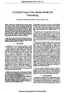
4. The common forecasting procedure, introduced in [5], is applied to get the forecasted values by each of three fuzzy time series models. 5. To defuzzify fuzzy values centroid method is used. Figure 2: The example of forecasting on six points of time series ts21.
6. Two step identification is used to choose the best forecasting fuzzy time series model. Below, we describe the results of the proposed algorithm for multiple time series. For this purpose the author’s software system was used. Figures 1, 2, 3, 4 show how proposed multiple time series forecasting algorithm processes some given time series. It is easy to see, that the chosen models well predict the time series tendencies. Numerical indicators of quality of the chosen models can also be considered as quite good. In comparison with the traditional time series model identification the applying of two step identification for forecasting of 91 time series showed the improvement of SMAPE for 40% (for two step time series model identification the average of out of sample SMAPE is equal 8.98%).
Figure 3: The example of forecasting on six points of time series ts22.
Figure 4: The example of forecasting on twelve points of time series ts38.
7. Conclusion In this paper the framework(algorithm) of multiple time series forecasting, based on fuzzy techniques, is proposed. The two-term additive decomposition of a time series, where the first term is a trend (expressed using the inverse F-transform components) and the second one is a residual vector is used. For the forecasting trend and residual vector three types of fuzzy models are used: a model with fuzzied time series values, a model with fuzzied first differences of time series values and a model with elementary fuzzy tendencies. A new criterion of similarity of behavior for given and predicted time series, based on fuzzy tendencies is used. As this criterion is model independent, it can be useful for a choosing of the best time series model of any types from the computational intelligence area.
Figure 5: The example of forecasting on four points of time series ts45. References [1] Abraham Otero. Future trends in data mining, http://biolab.uspceu.com/datamining/pdf/FutureTrends.pdf [2] Box, G. and Jenkins, G. (1970), Time Series Analysis: Forecasting and Control, HoldenDay, San Francisco. [3] Kendall, M. Time series, Translated from English, Yu. P. Lukashina. - Moscow: Finansy I statistica, 1981, 199 p. (rus). [4] Anderson T. W. (1971) Statistical Analysis of Time Series, New York: John Wiley and Sons, Inc., 1971. [5] Song, Q. (1993) Fuzzy time series and its models / Q. Song, B. Chissom // Fuzzy Sets and Systems. 1993, vol. 54, Ð . 269-277. [6] Chen, S. M. Forecasting enrollments based on high-order fuzzy time series / S.M. Chen // Cybernetics and Systems: An International Journal. 2002. - vol. 33, Ð . 1-16. [7] Hwang, J.R., Chen S.M. and Lee, C.H. 1998. Handling forecasting problem using fuzzy time series, Fuzzy Sets and Systems, 100, 217-228. [8] Novak, V., Stepnicka, M. Dvorak, A., Perfil-
Acknowledgements. The authors acknowledge that this paper was partially supported by by the projects no. 13-01-00324 and no. 14-07-00247 of the Russian Foundation for Basic Research.
Figure 1: The example of forecasting on six points of time series ts16.
1074
[9]
[10]
[11]
[12]
[13]
[14]
[15]
[16]
[17]
[18]
[19]
[20]
ieva, I. and Pavliska, V. (2010). Analysis of seasonal time series using fuzzy approach, International Journal of General Systems, 39, pp.305-328. Pedrycz W., Chen S.M. (Eds). (2013) Time Series Analysis, Modeling Applications, A Computational Intelligence Perspective (e-book Google). - Springer-Verlag, Berlin Heidelberg, 2013. - (Intelligent Systems Reference Library, Vol. 47). - 354-412 pp. Bardossy, A. Note on fuzzy regression / A Bardossy // Fuzzy Sets and Systems. - 1990. - Vol. 37 - Ð . 65-75. Wagner N., Michalewicz Z., Schellenberg S., Chiriac C., Mohais A. (2011) Intelligent techniques for forecasing multiple timeseries in realworld systems, International Journal of Intelligent Computing and Cybernetics, Vol. 4 Iss:3, pp.284-310. Yarushkina, N., Afanasieva, T., Perfilieva, I. Computational Intelligence in the analysis of time series. - ID "FORUM" : INFRA-M, Moscow, 2012, 160 pp. Tanaka, H. Linear regression analysis with fuzzy model / H. Tanaka, S. Uejima, K. Asai // IEEE Transactions on Systems, Man and Cybernetics. - 1982. - Vol. 12(6). - Ð . 903-907. Diamond, P. Fuzzy least squares / P. Diamond // Information Sciences. - 1988. - Vol. 46(3). Ð . 141-157. Tsenga, F. M. Fuzzy ARIMA model for forecasting the foreign exchange market / F. M. Tsenga, G. H. Tzengb, H. C. Yu // Fuzzy Sets and Systems. - 118 (2000) 9-19. Khashei, M. Improvement of Auto-Regressive Integrated Moving Average models using Fuzzy logic and Artificial Neural Networks / M. Khashei, M. Bijari , G. Rassi Ardali //Neurocomputing, 72(4), 2009, 956-967. Perfilieva, I., Yarushkina, N., Afanasieva, T., Romanov A. (2013) Time series analysis using soft computing methods, International Journal of General Systems, 42: 6, 687-705. Yaurshkina N.G.: Principes of the theory of fuzzy and hybrid systems. - Finances and statistics, Moscow (2004). Perfilieva, I. Fuzzy transforms: Theory and applications / I. Perfilieva // Fuzzy Sets and Systems - 2006. - Vol. 157. Mamdani, E.H., Assilian, S. An experiment in linguistic synthesis with a fuzzy logic controller, International Journal of Man-Machine Studies, 7(1):1-13, 1975.
1075