tween the âimplicitlyâ mapped coarse-grid and fine-grid TLM re- sponses. ..... The fine model employs a Johns matrix boundary [19]â[21] as an absorbing ...
IEEE TRANSACTIONS ON MICROWAVE THEORY AND TECHNIQUES, VOL. 53, NO. 9, SEPTEMBER 2005
2801
TLM-Based Modeling and Design Exploiting Space Mapping John W. Bandler, Fellow, IEEE, Ahmed S. Mohamed, Student Member, IEEE, and Mohamed H. Bakr, Member, IEEE
Abstract—In this paper, we study the use of space-mapping (SM) techniques within the transmission-line matrix (TLM) method environment. Previous work on SM relies on an “idealized” coarse model in the design process of a computationally expensive fine model. For the first time, we examine the case when the coarse model is not capable of providing an ideal optimal response. We exploit a coarse-grid TLM solver with relaxed boundary conditions. Such a coarse model may be incapable of satisfying design specifications and traditional SM may fail. Our approach, which exploits implicit SM (ISM) and the novel output SM (OSM), overcomes this failure. Dielectric constant, an expedient preassigned parameter, is first calibrated to roughly align the coarse and fine TLM models. Our OSM scheme absorbs the remaining deviation between the “implicitly” mapped coarse-grid and fine-grid TLM responses. Because the TLM simulations are on a fixed grid, response interpolation is crucial. We also create a database system to avoid repeating simulations unnecessarily. Our optimization routine employs a trust region methodology. The TLM-based design of an inductive post, a single-resonator filter, and a six-section H-plane waveguide filter illustrate our approach. In a few iterations, our coarse-grid TLM surrogate, with approximate boundary conditions, achieves a good design of the fine-grid TLM model in spite of poor initial responses. Our results are verified with MEFiSTo simulations. Index Terms—Computer-aided design (CAD), electromagnetic (EM) optimization, EM simulation, filter design, space mapping (SM), transmission-line matrix (TLM) method.
I. INTRODUCTION
T
HE space-mapping (SM) technique [1], [2] calibrates an enhanced “coarse” (simplified, fast, or low-fidelity) model to permit acceptable, near optimal design of a computationally expensive “fine” (practical, accurate, or high-fidelity) model with a minimal number of fine-model function evaluations [3]. This CAD methodology embodies the learning process of a designer [3].
Manuscript received August 13, 2004; revised February 1, 2005. This work was supported in part by the Natural Sciences and Engineering Research Council of Canada under Grant OGP0007239 and Grant, STPGP 269760, through the Micronet Network of Centres of Excellence and Bandler Corporation. The work of A.S. Mohamed is supported under the Ontario Graduate Scholarship (OGS) Program. J. W. Bandler is with Bandler Corporation, Dundas, ON, Canada L9H 5E7 and also with the Simulation Optimization Systems Research Laboratory, Department of Electrical and Computer Engineering, McMaster University, Hamilton, ON, Canada L8S 4K1. A. S. Mohamed is with the Simulation Optimization Systems Research Laboratory, Department of Electrical and Computer Engineering, McMaster University, Hamilton, ON, Canada L8S 4K1. M. H. Bakr is with the Department of Electrical and Computer Engineering, McMaster University, Hamilton, ON, Canada L8S 4K1. Digital Object Identifier 10.1109/TMTT.2005.854178
In previous implementations of SM technology, utilizing either an explicit input mapping [1], [2] or implicit [4] or output mappings [5], an “idealized” coarse model is assumed to be available. This coarse model, usually empirically based, provides a target optimal response with respect to (w.r.t.) the predefined design specifications while SM algorithms try to achieve a satisfactory “space-mapped” design . For the first time, we explore the SM methodology in the TLM [6] simulation environment. We design a CPU-intensive fine-grid TLM structure utilizing a coarse-grid TLM model with relaxed boundary conditions. Such a coarse model may not faithfully represent the fine-grid TLM model. Furthermore, it may not even satisfy the original design specifications. Hence, SM techniques such as the aggressive SM [2] will fail to reach a satisfactory solution. To overcome the aforementioned difficulty, we combine the implicit SM (ISM) [4] and output SM (OSM) [5] approaches. Parameter extraction (PE), equivalently called surrogate calibration, is responsible for constructing a surrogate of the fine model. As a preliminary PE step, the coarse model’s dielectric constant, a convenient preassigned parameter, is first calibrated. If the response deviation between the two TLM models is still large, an output SM scheme absorbs this deviation to make the updated surrogate represent the fine model. The subsequent surrogate optimization step is governed by a trust region strategy. The TLM simulator used in the design process is a Matlab [7] implementation. A set of design parameter values represents a point in the TLM simulation space. Because of the discrete nature of the TLM simulator, we employ an interpolation scheme to evaluate the responses, and possibly derivatives, at off-grid points [8], [9]. A database system is also created to avoid repeatedly invoking the simulator, to calculate the responses and derivatives, for a previously visited point. The database system is responsible for storage, retrieval, and management of all previously performed simulations [9]. Our proposed approach is illustrated through an inductive post, a single-resonator filter, and a six-section H-plane waveguide filter. We can achieve practical designs in a handful of iterations in spite of poor initial surrogate model responses. The results are verified using the commercial time-domain TLM simulator MEFiSTo [10]. In Section II, we review the basic concepts of TLM, implicit SM, output SM and trust region methodology. Our proposed approach is presented in Section III, explaining the surrogate calibration and surrogate optimization steps. We propose an algorithm in Section IV. Examples are illustrated in Section V, including the design of a six-section H-plane waveguide filter
0018-9480/$20.00 © 2005 IEEE
2802
IEEE TRANSACTIONS ON MICROWAVE THEORY AND TECHNIQUES, VOL. 53, NO. 9, SEPTEMBER 2005
with MEFiSTo verification. Conclusions and suggested future developments are drawn in Section VI.
Then, the optimized parameters are assigned to the fine model. This process repeats until the fine-model response is sufficiently close to the target response [4].
II. BASIC CONCEPTS D. Output Space Mapping (OSM)
A. Transmission-Line Matrix (TLM) Method The TLM method is a time and space discrete method for modeling electromagnetic (EM) phenomena [11]. A mesh of interconnected transmission lines model the propagation space [6]. The TLM method carries out a sequence of scattering and connection steps [11]. For the th nonmetalized node, the scattering relation is given by (1) where is the vector of incident impulses on the th node at is the vector of reflected impulses of the the th time step, th node at the th time step, and is the scattering matrix at the th node which is a function of the local dielectric constant . The reflected impulses become incident on neighboring nodes. For a nondispersive TLM boundary, a single time step is given by (2) where is the vector of incident impulses for all nodes at the th time step. The matrix is a block diagonal matrix whose th diagonal block is is the connection matrix and is the source excitation vector at the th time step. B. Design Problem Our design problem is given by (3) where is a vector of responses of the model, e.g., at selected frequency points. In a TLM-based enis a function of for all time steps . vironment, is the vector of fine-model design parameters and is a suitable objective function. For example, could be a minimax objective function with upper and lower is the optimal solution to be determined. specifications. C. Implicit Space Mapping (ISM) In the ISM approach, an auxiliary set of parameters is employed to calibrate the surrogate against the fine model. The surrogate can then be optimized to predict the next fine-model iterate [4]. In ISM, selected preassigned parameters denoted are extracted in an attempt to match the by coarse model to the fine model. Examples of preassigned parameters in a microwave structure are dielectric constant and substrate height [12]. With these parameters fixed in the fine model, the calibrated (implicitly mapped) coarse model denoted , at the th iteration, is optimized w.r.t. by as the design parameters (4)
Although the fine and coarse models usually share the same physical background, they are still two different models and a deviation between them in the response space (i.e., the range) always exists. This deviation cannot be compensated by only manipulating the parameters (i.e., the domain) through the regis originally proposed to fine ular SM. OSM tune the residual response deviation [5] between the fine model and its surrogate, in the final stages. In this case, the surrogate incorporates a faithful coarse model and could be given by the following composite function: (5) E. Trust Region (TR) Methods [13] TR strategies are employed to assure convergence of an optimization algorithm and to stabilize the iterative process [14]. The TR approach was first introduced in the context of SM with the aggressive SM technique in [15]. The aim of TR methods is to adjust the length of the step taken at each iteration, in an optimization routine, based on how well an approximate model predicts the objective function of the actual model. The approximate model is trusted to represent the objective function only within a region of specific radius around the current iteration. The local-model minimum inside the trust region is found by solving a TR subproblem. If the model minimum achieves sufficient actual reduction in the objective function, the TR size is increased. If insufficient reduction is achieved, the TR is reduced. Otherwise, the TR is kept unchanged. III. PROPOSED APPROACH In this study, we propose an approach to create a surrogate of the fine model that exploits an input implicit mapping (model domain) and encompasses the response deviation between the fine model and its surrogate (model range) through an output mapping. The proposed output SM scheme absorbs possible response misalignments through a response linear transformation (shift and scale). Fig. 1 describes a conceptual scheme for combining an input parameter mapping (implicit in our case) along with an output response mapping. At the th iteration, a surrogate of the fine model is given by
(6) is the preassigned parameter vector whose value where is the evaluation of the implicit mapping at . The scaling diand the shifting vector agonal matrix are the output mapping parameters. The preassigned parameters and the output mapping parameters are evaluated through a surrogate calibration, i.e., the parameter extraction process.
BANDLER et al.: TLM-BASED MODELING AND DESIGN EXPLOITING SPACE MAPPING
2803
B. Surrogate Optimization (Prediction) We optimize a suitable objective function of the surrogate (6) in effort to obtain a solution of (3). We utilize the TR methodology to find the step in the fine space at the th iteration [12], [14]
(10)
Fig. 1. ISM and OSM concepts. We calibrate the surrogate against the fine model utilizing the preassigned parameters x , e.g., dielectric constant, and the output response mapping parameters: the scaling matrix � and the shifting vector .
where is the trust region size at the th iteration. The tentais accepted as a successful step in the fine-model tive step parameter space if there is a reduction of the fine model objective function, otherwise the step is rejected
A. Parameter Extraction (Surrogate Calibration) The PE optimization process is a key element in any SM algorithm. It is performed here to align the surrogate (6) with the fine model by calibrating the mapping(s) parameters. The deviation between the fine model and the surrogate reis given by sponses at the current fine-model point (7) At the th iteration, mapping parameters
is first extracted keeping the output fixed as follows:
(11) The TR radius is updated according to [14]. C. Stopping Criteria The algorithm stops when one of the following stopping criteria is satisfied. 1) A predefined maximum number of iterations is reached. 2) The step length taken by the algorithm is sufficiently small [18], e.g., , where is a userdefined small number. 3) The trust region radius reaches a minimum allowed , i.e., . value IV. ALGORITHM
(8) where a multipoint PE (MPE) scheme [16], [17] is employed. We calibrate the surrogate model against the fine model at a set of points with , where is the number of fine-model points utilized at the th PE iteration. At each PE iteration, we initially set . Then, some fine-model points of the previous successful iterates are included into the set and hence more information about the fine model could be utilized. Then, we calibrate the surrogate by manipulating at and to absorb the response deviation
(9) and are ideally and , respectively. The PE (9) is penalized such that and remain close to their ideal values. and are user-defined weighting factors. A suitable norm, denoted by , is utilized in (8) and (9), e.g., the norm.
Given . Comment. The initial trust region radius is and the nominal preassigned parameter value is Step 1) Initialize and . Step 2) Solve (4) to find the initial surrogate optimizer. Comment. The initial surrogate is the coarse model Step 3) Evaluate the fine model response . Step 4) Find surrogate parameters through PE (8) and (9). Step 5) Obtain by solving (10). Step 6) Evaluate . Step 7) Set according to (11). Step 8) Update according to the criterion in [14]. Step 9) If the stopping criterion is satisfied (see Section III-C), terminate. Step 10) If the TR step is successful, increment and go to Step 4), else go to Step 5). V. EXAMPLES A Matlab implementation of a two-dimensional (2-D) TLM simulator is utilized. We employ the dielectric constant as a ) for the whole region scalar preassigned parameter (i.e., in all of the coming examples.
2804
IEEE TRANSACTIONS ON MICROWAVE THEORY AND TECHNIQUES, VOL. 53, NO. 9, SEPTEMBER 2005
Fig. 3. Progression of the optimization iterates for the inductive post on the are in millimeters). fine modeling grid ( and
D
W
Fig. 2. Inductive post in a parallel-plate waveguide. (a) Three-dimensional plot. (b) Cross section with magnetic side walls.
A. Inductive Obstacle in a Parallel-Plate Waveguide Fig. 2 shows an inductive post centered in a parallel-plate and width waveguide with fixed dimensions. Thickness of the inductive obstacle are design parameters. We are studying the TEM mode propagation. Due to symmetry, only half of the structure is simulated. We use the fine model with a square cell mm, while the coarse model utilizes a square cell mm. We utilized 21 frequency points in the frequency range 2.5 GHz. The objective function is defined to 0.1 GHz and of a given match the real and imaginary parts of target response. An interpolation scheme is used [8] in optimizing the surrogate (calibration and prediction steps). The least-squares Levenberg–Marquardt algorithm available in Matlab [7] is utilized to solve both the PE problem and the TR subproblem in each iteration. The PE is designed to match the fine model with the surrogate at the current point in both (8) and (9), i.e., . and are set to zero. The algorithm converges in seven iterations. The progression of the optimization iterates on the fine modeling grid is shown in Fig. 3. The target, fine-model, and surrogate responses at the initial and the final iterations for are shown in Fig. 4. Fig. 5 illustrates the reduction of the fine model and the corresponding surrogate objective functions along iterations. The optimization results are summarized in Table I.
Fig. 4. Optimal target response (—), the fine-model response (�), and the j) at (a) the initial design surrogate response (- - -) for the inductive post (j and (b) the final design.
S
Our proposed approach, without the database system, takes 34 min versus 68 min for direct optimization. Utilizing the database system reduces the execution time to 4 min.
BANDLER et al.: TLM-BASED MODELING AND DESIGN EXPLOITING SPACE MAPPING
2805
Fig. 5. Reduction of the objective function (U ) of the fine model (—) and the surrogate (- - -) for the inductive post. TABLE I OPTIMIZATION RESULTS FOR THE INDUCTIVE POST
Fig. 6. Statistical analysis for the real and imaginary parts of S of the inductive post with 2% relative tolerances (a) using the fine model and (b) using the surrogate at the final iteration of the optimization. One hundred outcomes are used.
A statistical analysis of the surrogate at the final design is carried out with 100 samples. The relative tolerance used is 2%. The results show good agreement between the fine model (75 min for 100 outcomes) and its surrogate (7 min for 100 outfor both the fine comes). The real and imaginary parts of model and its surrogate at the final design are shown in Fig. 6. B. Single-Resonator Filter A single-resonator filter is shown in Fig. 7. The design parameters are the resonator length and the septum width . The rectangular waveguide width and length are fixed as shown in with a cutoff frequency Fig. 7. The propagating mode is of 2.5 GHz. We use the fine model with a square cell mm, while the coarse model utilizes a square cell mm. The frequency range is 3.0 GHz 5.0 GHz with steps of 0.1 GHz. The fine model employs a Johns matrix boundary [19]–[21] as an absorbing boundary condition while the coarse model utilizes a single impulse reflection coefficient calculated at the
Fig. 7.
Topology of the single-resonator filter.
center frequency (4.0 GHz). Hence, we do not need to calculate the Johns matrix for the coarse model each time we change
2806
IEEE TRANSACTIONS ON MICROWAVE THEORY AND TECHNIQUES, VOL. 53, NO. 9, SEPTEMBER 2005
Fig. 9. Reduction of the objective function (U ) of the fine model (—) and the surrogate (- - -) for the single-resonator filter.
Fig. 8. Surrogate response (- - � - -) and the corresponding fine model response (— � —) at (a) the initial design and (b) the final design (using linear interpolation) for the single-resonator filter.
. This introduces another source of inaccuracy in the coarse model. A minimax objective function is used in the design process with upper and lower design specifications for
GHz
GHz
for
GHz
GHz
for
GHz
GHz
Fig. 10. Progression of the optimization iterates for the single-resonator filter on the fine modeling grid (d and W are in millimeters). TABLE II OPTIMIZATION RESULTS FOR THE SINGLE-RESONATOR FILTER
(12)
The Matlab [7] least-squares Levenberg–Marquardt algorithm solves the PE problem. The TR subproblem (10) is solved by the minimax routine described in [22]. An interpolation scheme with database system is used [8]. The surrogate is calibrated to match the fine model at the last two points in (8) and the current point in (9). The weighting factors are set to and . The algorithm converges in five iterations to an optimal fine model response although the coarse model initially exhibits a very poor response [see Fig. 8(a)]. Fig. 8(b) depicts the fine-grid TLM response along with its surrogate response at the final design. The reduction of the objective function of the fine model and the surrogate versus iteration and the progres-
sion of the optimization iterates are shown in Figs. 9 and 10, respectively. The optimal design reached by the algorithm is given by 32.99 mm and mm (see Table II for the optimization summary). Our proposed approach, without the database system, takes 88 min versus 172 min for direct optimization. Utilizing the database system reduces the execution time to 15 min.
BANDLER et al.: TLM-BASED MODELING AND DESIGN EXPLOITING SPACE MAPPING
2807
Fig. 12. Six-section H-plane waveguide filter. (a) The 3-D view. (b) One half of the 2-D cross section. (c) The equivalent empirical circuit model.
Fig. 11. Final design reached by the algorithm (— � —) versus the simulation results using MEFiSTo 2-D with the rubber cell feature (—) for the single-resonator filter (a) jS j and (b) jS j.
We utilize the time-domain TLM simulator MEFiSTo [10] to verify our results. We employ the rubber cell feature [10] in MEFiSTo to examine our interpolation scheme. Using the TLM conformal (rubber) cell [23], the dimensions of the underlying structure, which are not located at multiple integers of the mesh size, will not be shifted to the closest cell boundary. Rather, a change in the size and shape of the TLM boundary cell, due to an irregular boundary position, is translated into a change in its input impedance at the cell interface with a regular computational mesh [23]. Fig. 11 shows a good agreement between the interpolated results of the final design obtained from our algorithm and the MEFiSTo simulation utilizing the rubber cell. C. Six-Section H-Plane Waveguide Filter We consider the six-section H-plane waveguide filter [24], [25] [see the 3-D view and 2-D cross section in Fig. 12(a) and (b), respectively]. A waveguide with a width of 1.372 in (3.485 cm) is used. The propagation mode is with a cutoff frequency of 4.3 GHz. The six-waveguide sections are separated by seven H-plane septa, which have a finite thickness of 0.0245 in (0.6223 mm). The design parameters are the
three waveguide-section lengths and and the septa widths , and . A minimax objective function is employed with upper and lower design specifications given by for for for
GHz
GHz GHz
GHz
(13)
We use the fine model with a square cell mm. The number of TLM cells in the and directions are and , respectively. A Johns matrix boundary [19]–[21] is used as a dispersive absorbing boundary conditime steps. We utilize 23 points in the tion with 10.0 GHz. We consider the frequency range 5.0 GHz filter design using two different coarse models: empirical coarse model and coarse-grid TLM model. In both cases, we use the least-squares Levenberg–Marquardt algorithm in Matlab [7] for the PE. A linear interpolation scheme with a database system is utilized for the surrogate optimization using the minimax routine given in [22]. The PE is designed to match the fine model with its surrogate utilizing the most recent three points in (8) and the current point in (9). We set the weighting factors to and . Case 1: Empirical Coarse Model: A coarse model with lumped inductances and dispersive transmission-line sections is utilized. We simplify formulas due to Marcuvitz [26] for the inductive susceptances corresponding to the H-plane septa.
2808
IEEE TRANSACTIONS ON MICROWAVE THEORY AND TECHNIQUES, VOL. 53, NO. 9, SEPTEMBER 2005
TABLE III INITIAL AND FINAL DESIGNS FOR THE SIX-SECTION H-PLANE WAVEGUIDE FILTER DESIGNED USING THE EMPIRICAL COARSE MODEL
Fig. 14. Reduction of the objective function (U ) of the fine model (—) and the surrogate (- - -) for the six-section H-plane waveguide filter designed using the empirical coarse model.
Fig. 15. Final design reached by the algorithm (—�—) compared with MEFiSTo 2-D simulation with the rubber cell feature (—) for the six-section H-plane waveguide filter designed using the empirical coarse model.
Fig. 13. Surrogate response (- - � - -) and the corresponding fine model response (— � —) at (a) the initial design and (b) the final design (using linear interpolation) for the six-section H-plane waveguide filter designed using the empirical coarse model.
They are connected to the transmission-line sections through circuit theory [27]. The model is implemented and simulated in the Matlab [7] environment. Fig. 12(c) shows the empirical circuit model. The algorithm converges to an optimal solution in ten iterations. The initial and final designs are shown in Table III. The
. The initial and final responses for the final value of fine model and its surrogate are illustrated in Fig. 13. Fig. 14 depicts the reduction of objective function of the fine model and its surrogate. The final design response using our algorithm is compared with MEFiSTo in Fig. 15. Case 2: Coarse-Grid TLM Model: We utilize a coarse-grid TLM model with a square cell mm. The and number of TLM cells in the and directions are , respectively. The number of time steps is time steps. A single impulse reflection coefficient calculated at the center frequency (7.5 GHz) is utilized. We have three sources of inaccuracy of the coarse-grid TLM model, namely, the coarser grid, the inaccurate absorbing boundary conditions and the reduced number of time steps. This reduces the computation time of the coarse model versus the fine model. We apply our algorithm. Despite the poor starting surrogate response [see Fig. 16(a)], the algorithm reaches an optimal solution in 8 iterations. The initial and final designs are shown in . The initial and final Table IV. The final value of responses for the fine model and its surrogate are illustrated in
BANDLER et al.: TLM-BASED MODELING AND DESIGN EXPLOITING SPACE MAPPING
2809
Fig. 17. Reduction of the objective function (U ) of the fine model (—) and the surrogate (- - -) for the six-section H-plane waveguide filter designed using the coarse-grid TLM model.
Fig. 16. Surrogate response (- - � - -) and the corresponding fine model response (— � —) at (a) the initial design and (b) the final design (using linear interpolation) for the six-section H-plane waveguide filter designed using the coarse-grid TLM model. Fig. 18. Final design reached by the algorithm (—�—) compared with MEFiSTo 2-D simulation with the rubber cell feature (—) for the six-section H-plane waveguide filter designed using the coarse-grid TLM model. TABLE IV INITIAL AND FINAL DESIGNS FOR THE SIX-SECTION H-PLANE WAVEGUIDE FILTER DESIGNED USING THE COARSE-GRID TLM MODEL TABLE V OUR APPROACH WITH/WITHOUT DATABASE SYSTEM VERSUS DIRECT OPTIMIZATION FOR THE SIX-SECTION H-PLANE WAVEGUIDE FILTER DESIGNED USING COARSE-GRID TLM MODEL
Fig. 16. The reduction of the objective function of the fine model and its surrogate is shown in Fig. 17. The final design response obtained using our algorithm is compared with MEFiSTo simulation in Fig. 18. It shows good agreement.
Using the proposed approach, the optimization time is reduced by 66% w.r.t. direct optimization, as shown in Table V. The dynamically updated database system, implemented in the algorithm, reduces the optimization time even more, as reported in Table V. The run time for the PE process, surrogate optimization, and fine-model simulation of our proposed approach are 15, 4, and 58 min, respectively.
2810
IEEE TRANSACTIONS ON MICROWAVE THEORY AND TECHNIQUES, VOL. 53, NO. 9, SEPTEMBER 2005
VI. CONCLUSION For the first time, we investigate the SM approach to modeling and design when the coarse model does not faithfully represent the fine model. In this study, a coarse-grid TLM model with relaxed boundary conditions is utilized as a coarse model. Such a model may provide a response that deviates significantly from the original design specifications and, hence, previous SM implementations may fail to reach a satisfactory solution. We propose a technique exploiting implicit SM and output SM. The dielectric constant, a convenient preassigned parameter, is first calibrated for a rough (preprocessing) alignment between the coarse and fine TLM models. Output SM absorbs the remaining response deviation between the TLM fine-grid model and the implicitly mapped TLM coarse-grid model (the surrogate). To accommodate the discrete nature of our EM simulator, we designed the algorithm to have interpolation and dynamically updated database capabilities, which is key to efficient design automation. Our approach is illustrated through the TLM-based design of an inductive post, a single-resonator filter, and a six-section H-plane waveguide filter. Our algorithm converges to a good design for the fine-grid TLM model in spite of poor initial behavior of the coarse-grid TLM surrogate. We consider our results to be promising. Utilizing, as preassigned parameters, different dielectric constants for different regions of the underlying microwave structure is addressed here but not implemented. Incorporating Jacobians in the PE process to improve the construction of the surrogate, e.g., exploiting adjoint variable methods, needs future investigation.
ACKNOWLEDGMENT The authors would like to thank Dr. W. J. R. Hoefer, University of Victoria, Victoria, BC, Canada, for useful discussions and making the Faustus MEFiSTo software available. They would also like to thank Dr. K. Madsen, Technical University of Denmark, Lyngby, Denmark, for continued collaboration. They also acknowledge discussions and technical input from S. A. Dakroury, formerly with McMaster University, and thank Dr. S. Koziel of McMaster University for his insightful comments on our manuscript.
REFERENCES [1] J. W. Bandler, R. M. Biernacki, S. H. Chen, P. A. Grobelny, and R. H. Hemmers, “Space mapping technique for electromagnetic optimization,” IEEE Trans. Microw. Theory Tech., vol. 42, no. 12, pp. 2536–2544, Dec. 1994. [2] J. W. Bandler, R. M. Biernacki, S. H. Chen, R. H. Hemmers, and K. Madsen, “Electromagnetic optimization exploiting aggressive space mapping,” IEEE Trans. Microw. Theory Tech., vol. 43, no. 12, pp. 2874–2882, Dec. 1995. [3] J. W. Bandler, Q. Cheng, S. A. Dakroury, A. S. Mohamed, M. H. Bakr, K. Madsen, and J. Søndergaard, “Space mapping: The state of the art,” IEEE Trans. Microw. Theory Tech., vol. 52, no. 1, pp. 337–361, Jan. 2004.
[4] J. W. Bandler, Q. S. Cheng, N. K. Nikolova, and M. A. Ismail, “Implicit space mapping optimization exploiting preassigned parameters,” IEEE Trans. Microw. Theory Tech., vol. 52, no. 1, pp. 378–385, Jan. 2004. [5] J. W. Bandler, Q. S. Cheng, D. Gebre-Mariam, K. Madsen, F. Pedersen, and J. Søndergaard, “EM-based surrogate modeling and design exploiting implicit, frequency and output space mappings,” in IEEE MTT-S Int. Microwave Symp. Dig., Philadelphia, PA, Jun. 2003, pp. 1003–1006. [6] W. J. R. Hoefer, “The transmission-line matrix method—Theory and applications,” IEEE Trans. Microw. Theory Tech., vol. MTT-33, no. 10, pp. 882–893, Oct. 1985. [7] Matlab™, 2002. Version 6.5. [8] J. W. Bandler, R. M. Biernacki, S. H. Chen, L. W. Hendrick, and D. Omeragic, “Electromagnetic optimization of 3-D structures,” IEEE Trans. Microw. Theory Tech., vol. 45, no. 5, pp. 770–779, May 1997. [9] P. A. Grobelny, “Integrated numerical modeling techniques for nominal and statistical circuit design,” Ph.D. dissertation, Dept. Elect. Comput. Eng., McMaster Univ., Hamilton, ON, Canada, 1995. [10] MEFiSTo-3D Pro, 2003. Version 3.0. [11] M. H. Bakr, P. P. M. So, and W. J. R. Hoefer, “The generation of optimal microwave topologies using time-domain field synthesis,” IEEE Trans. Microw. Theory Tech., vol. 50, no. 11, pp. 2537–2544, Nov. 2002. [12] J. W. Bandler, M. A. Ismail, and J. E. Rayas-Sánchez, “Expanded space mapping EM-based design framework exploiting preassigned parameters,” IEEE Trans. Circuits Syst. I, Fundam. Theory Appl., vol. 49, no. 12, pp. 1833–1838, Dec. 2002. [13] A. R. Conn, N. I. M. Gould, and P. L. Toint, Trust-Region Methods. Philadelphia, PA: SIAM and MPS, 2000. [14] N. M. Alexandrov, J. E. Dennis, Jr., R. M. Lewis, and V. Torczon, “A trust-region framework for managing the use of approximation models in optimization,” Struct. Optim., vol. 15, pp. 16–23, 1998. [15] M. H. Bakr, J. W. Bandler, R. M. Biernacki, S. H. Chen, and K. Madsen, “A trust region aggressive space mapping algorithm for EM optimization,” IEEE Trans. Microw. Theory Tech., vol. 46, no. 12, pp. 2412–2425, Dec. 1998. [16] J. W. Bandler, R. M. Biernacki, and S. H. Chen, “Fully automated space mapping optimization of 3D structures,” in IEEE MTT-S Int. Microwave Symp. Dig., San Francisco, CA, Jun. 1996, pp. 753–756. [17] J. W. Bandler, R. M. Biernacki, S. H. Chen, and D. Omeragic, “Space mapping optimization of waveguide filters using finite element and mode-matching electromagnetic simulators,” Int. J. RF Microwave Computer-Aided Eng., vol. 9, no. 1, pp. 54–70, Jan. 1999. [18] J. Søndergaard, “Optimization using surrogate models—by the space mapping technique,” Ph.D. dissertation, Dept. Inform. Math. Modeling, Tech. Univ. Denmark, Lyngby, Denmark, 2003. [19] P. B. Johns and K. Akhtarzad, “The use of time domain diakoptics in time discrete models of fields,” Int. J. Num. Methods Eng., vol. 17, pp. 1–14, 1981. , “Time domain approximations in the solution of fields by time [20] domain diakoptics,” Int. J. Num. Methods Eng., vol. 18, pp. 1361–1373, 1982. [21] C. Eswarappa, G. I. Costache, and W. J. R. Hoefer, “Transmission line matrix modeling of dispersive wide-band absorbing boundaries with time-domain diakoptics for S -parameter extraction,” IEEE Trans. Microw. Theory Tech., vol. 38, no. 4, pp. 379–386, Apr. 1990. [22] K. Madsen, H. B. Nielsen, and J. Søndergaard, “Robust subroutines for non-linear optimization,” Denmark Tech. Univ., Lyngby, Denmark, Tech. Rep. IMM-REP-2002-02, , 2002. [23] P. P. M. So and W. J. R. Hoefer, “Locally conformal cell for two-dimensional TLM,” in IEEE MTT-S Int. Microwave Symp. Dig., Philadelphia, PA, Jun. 2003, pp. 977–980. [24] G. L. Matthaei, L. Young, and E. M. T. Jones, Microwave Filters, Impedance-Matching Networks, and Coupling Structures, 1st ed. New York: McGraw-Hill, 1964. [25] M. H. Bakr, J. W. Bandler, N. Georgieva, and K. Madsen, “A hybrid aggressive space mapping algorithm for EM optimization,” IEEE Trans. Microw. Theory Tech., vol. 47, no. 12, pp. 2440–2449, Dec. 1999. [26] N. Marcuvitz, Waveguide Handbook, 1st ed. New York: McGraw-Hill, 1951, p. 221. [27] M. Pozar, Microwave Engineering, 2nd ed. New York: Wiley, 1998.
BANDLER et al.: TLM-BASED MODELING AND DESIGN EXPLOITING SPACE MAPPING
John W. Bandler (S’66–M’66–SM’74–F’78) was born in Jerusalem on November 9, 1941. He received the B.Sc. (Eng.), Ph.D., and D.Sc. (Eng.) degrees from the University of London, London, U.K., in 1963, 1967, and 1976, respectively. In 1966, he joined Mullard Research Laboratories, Redhill, Surrey, U.K. From 1967 to 1969, he was a Post-Doctorate Fellow and Sessional Lecturer with the University of Manitoba, Winnipeg, MB, Canada. In 1969, he joined McMaster University, Hamilton, ON, Canada, where he has served as Chairman of the Department of Electrical Engineering and Dean of the Faculty of Engineering. He is currently Professor Emeritus in Electrical and Computer Engineering and directs research in the Simulation Optimization Systems Research Laboratory. He was President of Optimization Systems Associates, Inc. (OSA), Dundas, ON, Canada, which he founded in 1983, until November 20, 1997, the date of acquisition of OSA by the Hewlett-Packard Company (HP). OSA implemented a first-generation yield-driven microwave CAD capability for Raytheon in 1985, followed by further innovations in linear and nonlinear microwave CAD technology for the Raytheon/Texas Instruments Joint Venture MIMIC Program. OSA introduced the computer-aided engineering (CAE) systems RoMPE in 1988, HarPE in 1989, OSA90 and OSA90/hope in 1991, Empipe in 1992, and Empipe3D and EmpipeExpress in 1996. OSA created empath in 1996, marketed by Sonnet Software, Inc. He is currently President of Bandler Corporation, Dundas, ON, Canada, which he founded in 1997. He has authored or coauthored over 370 papers from 1965 to 2005. He contributed to Modern Filter Theory and Design (New York: Wiley-Interscience, 1973) and Analog Methods for Computer-aided Analysis and Diagnosis (New York: Marcel Dekker, 1988). Four of his papers have been reprinted in Computer-Aided Filter Design (New York: IEEE Press, 1973), one in each of Microwave Integrated Circuits (Norwood, MA: Artech House, 1975), Low-Noise Microwave Transistors and Amplifiers (New York: IEEE Press, 1981), Microwave Integrated Circuits, 2nd ed.(Norwood, MA: Artech House, 1985), Statistical Design of Integrated Circuits (New York: IEEE Press, 1987), and Analog Fault Diagnosis (New York: IEEE Press, 1987). He joined the Editorial Boards of the International Journal of Numerical Modeling (1987), the International Journal of Microwave and Millimeterwave Computer-Aided Engineering (1989), and Optimization Eng. in 1998. He was Guest Editor of the International Journal of Microwave and Millimeter-Wave Computer-Aided Engineering Special Issue on Optimization-Oriented Microwave CAD (1997). He was guest co-editor of the Optimization and Engineering Special Issue on Surrogate Modeling and Space Mapping for Engineering Optimization (2001). Dr. Bandler is a Fellow of the Canadian Academy of Engineering, the Royal Society of Canada, the Institution of Electrical Engineers (U.K.), and the Engineering Institute of Canada. He is a member of the Association of Professional Engineers of the Province of Ontario (Canada) and a member of the Massachusetts Institute of Technology (MIT) Electromagnetics Academy. He was an Associate Editor of the IEEE TRANSACTIONS ON MICROWAVE THEORY AND TECHNIQUES (T-MTT) from 1969 to 1974 and has continued serving as a member of the Editorial Board. He was Guest Editor of the T-MTT Special Issue on Computer-Oriented Microwave Practices (1974) and Guest Coeditor of the IEEE T-MTT Special Issue on Process-Oriented Microwave CAD and Modeling (1992). He was Guest Editor of the IEEE T-MTT Special Issue on Automated Circuit Design Using Electromagnetic Simulators (1997). He was Guest Coeditor of the IEEE T-MTT Special Issue on Electromagnetics-Based Optimization of Microwave Components and Circuits (2004). He has served as chair of the MTT-1 Technical Committee on Computer-Aided Design. He was the recipient of the 1994 Automatic Radio Frequency Techniques Group (ARFTG) Automated Measurements Career Award and the 2004 Microwave Application Award presented by the IEEE MTT-S.
2811
Ahmed S. Mohamed (S’00) was born in Cairo, Egypt, in 1973. He received the B.Sc. degree with distinction (honors) in electronics and communications engineering and the M.S. degree in engineering mathematics from Cairo University, Cairo, Egypt, in 1995 and 2000, respectively, and the Ph.D. degree from McMaster University, Hamilton, ON, Canada, in 2005. His master’s thesis topic was about time series forecasting using mixtures of neural networks and conventional models. In September 1995, he joined the Department of Engineering Mathematics and Physics, Faculty of Engineering, Cairo University, as a Teaching and Research Assistant. In September 2000, he joined the Department of Electrical and Computer Engineering, McMaster University. His current research is carried out in the Simulation Optimization Systems Research Laboratory. He is interested in electromagnetic optimization methods, microwave computer-aided design, neural network applications, and modeling of microwave circuits. Mr. Mohamed was a recipient of an Ontario Graduate Scholarship (OGS) for two consecutive academic years 2003–2004 and 2004–2005.
Mohamed H. Bakr (S’98–M’00) received the B.Sc. degree in electronics and communications engineering with distinction (honors) and the M.S. degree in engineering mathematics from Cairo University, Cairo, Egypt, in 1992 and 1996, respectively, and the Ph.D. degree from McMaster University, Hamilton, ON, Canada, in 2000. In 1997, he was a student intern with Optimization Systems Associates, Inc. (OSA), Dundas, ON, Canada. From 1998 to 2000, he worked as a Research Assistant with the Simulation Optimization Systems (SOS) Research Laboratory, McMaster University. In November 2000, he joined the Computational Electromagnetics Research Laboratory (CERL), University of Victoria, Victoria, BC, Canada as an NSERC Post Doctoral Fellow. His research areas of interest include optimization methods, computer-aided design and modeling of microwave circuits, neural network applications, smart analysis of microwave circuits, and efficient optimization using time-/frequency-domain methods. He is currently an Assistant Professor with the Department of Electrical and Computer Engineering, McMaster University. Dr. Bakr was a recipient of the Premier’s Research Excellence Award (PREA) from the Province of Ontario, Canada, in 2003.