Kraus and Ertl [7] considered rectilinear data sets and piecewise trilinear ..... and Hans Hagen, editors, IEEE Visualization '98, pages 51â58, ACM Press, New ...
Topology-based Transfer Function Design Gunther H. Weber, Gerik Scheuermann AG Graphische Datenverarbeitung und Computergeometrie, FB Informatik, University of Kaiserslautern, Erwin-Schr¨odinger-Straße, 67663 Kaiserslautern, Germany
Abstract
pear/disappear in a surface component, or disjoint surface components merge at saddles. Values and locations where such changes occur are determined and used to aid a user in data exploration. Instead of using the resulting set of critical isovalues as indicator for which isovalues expressive isosurfaces result, it is possible to use them to construct a transfer function that highlights topological properties of a scalar data set. DVR commonly uses trilinear interpolation commonly within cells. Thus, critical isovalues extracted by Weber et al. [10] are also meaningful in a volume rendering context. We use the resulting list of critical isovalues to design transfer functions based on the work presented by Fujishiro et al. [3, 5]. We generate transfer functions that assign small opacity to all scalar values except those close to critical isovalues. Colors are assigned using an HLS color model and varying the hue component for different scalar values such that it changes more rapidly close to critical isovalues.
Direct Volume Rendering (DVR) is commonly used to visualize scalar fields. Quality and significance of rendered images depend on the choice of an appropriate transfer function that assigns optical properties (e.g., color and opacity) to scalar values. We present a method that automatically generates a transfer function based on the topological behavior of a scalar field. We find a set of critical isovalues for which the topology of an isosurface, i.e., a surface representing all locations where the scalar field assumes a certain value v, changes. Then we generate a transfer function that emphasizes scalar values around those critical isovalues. Images rendered using the resulting transfer function reveal the fundamental topological structure of a scalar data set.
1. Introduction
2.
Direct Volume Rendering visualizes a three-dimensional (3D) scalar field by using a transfer function to map scalar values to optical properties (e.g., color and opacity) and rendering the resulting image. This transfer function presents a user with an additional parameter that influences a resulting visualization. However, quality and significance of the resulting visualization hinge on a sensible choice of the transfer function. Transfer functions are commonly determined manually by trial and error which is time-consuming and prone to errors. Several attempts were made to analyze a data set and generate appropriate transfer functions automatically to aid a user in the visualization process. Pfister et al. [9] give an overview over several techniques and compare results with manually chosen transfer functions. Apart from DVR, isosurfaces are most commonly used to visualize scalar fields f (x, y, z). An isosurface represents all locations in 3D space, where f assumes a given isovalue v, i.e., where f = v holds. By varying the isovalue v, it is possible to visualize the entire scalar field. Like choosing appropriate transfer functions, determining isovalues where “interesting” isosurface behavior occurs is difficult. Weber et al. [10] have considered the topological properties of a piecewise trilinear scalar field to determine for which isovalues relevant isosurface behavior occurs. All fundamental changes are tracked: Closed surface components emerge or vanish at local minima or maxima, and the genus of an isosurface changes, i.e., holes ap-
Related Work
Few authors utilize topological analysis for scalar field visualization. Bajaj et al. [2] developed a technique to visualize topology to enhance visualizations of trivariate scalar fields. Their method employs a C 1 -continuous interpolation scheme for rectilinear grids, and it detects critical points of a scalar field, i.e., points where the gradient of the scalar field vanishes. Subsequently, integral curves (tangent curves) are traced starting from locations close to saddle points. These integral curves are superimposed onto volume-rendered images to convey structural information of the scalar field. Fujishiro et al. [3] used a hyper-Reeb graph for exploration of scalar fields. A Reeb graph encodes topology of a surface. The hyper-Reeb graph encodes changes of topology in an extracted isosurface. For each isovalue that corresponds to an isosurface topology change, a node exists in the hyper-Reeb graph containing a Reeb graph encoding the topology of that isosurface. Fujishiro et al. [3] construct a hyper-Reeb graph using “focusing with interval volumes,” an iterative approach that finds a subset of all critical isovalues , which had been introduced by Fujishiro and Takeshima [4]. The hyper-Reeb graph can be used, for example, for automatic generation of transfer functions. Fujishiro et al. [5] extended this work and used a hyperReeb graph for exploration of volume data. In addition to automatic transfer function design, their extended method 1
allows them to generate translucent isosurfaces between critical isovalues. Critical point behavior is also important in the context of data simplification to preserve important features of a data set. Bajaj and Schikore [1] extended previous methods to develop a compression scheme preserving topological features. Their approach detects critical points of a piecewise linear bivariate scalar field f (x, y). In their approach, “critical vertices” are those vertices for which the “normal space” of the surrounding triangle platelet contains the vector (0, 0, 1). Integral curves are computed by tracing edges of triangles along a “ridge” or “channel.” Bajaj and Schikore’s method incorporates an error measure and can be used for topology-preserving mesh simplification. Gerstner and Pajarola [6] defined a bisection scheme that enumerates all grid points of a rectilinear grid in a tetrahedral hierarchy. Using piecewise linear interpolation in tetrahedra, critical points can be detected. Data sets are simplified by specifying a traversal scheme that descends only as deep into the tetrahedral hierarchy as necessary to preserve topology within a certain error bound. This method incorporates heuristics that assign importance values to topological features, enabling a controlled topology simplification. Kraus and Ertl [7] considered rectilinear data sets and piecewise trilinear interpolation. Their technique partitions rectilinear cells into tetrahedra and uses critical points of linear interpolation to guide them in sub-sampling scheme when attempting to preserve topology. Weber et al. [10] use critical point analysis to help a user in exploring a scalar data set using isosurfaces. By presenting a user with a list of critical isovalues of a piecewise trilinear scalar field they provide important “navigational aids” for the visualization process. A user can explore a data set by examining isosurface behavior close to critical isovalues. Pfister et al. [9] review recent approaches to automated transfer function design. They compare transfer functions resulting from a variety of automated schemes to manually chosen transfer functions.
3.
Detecting Critical Isovalues
Our goal is to detect critical isovalues of a piecewise trilinear scalar field. For a C 1 -continuous function f , critical points occur where the gradient ∇f assumes a value of zero, i.e., ∇f = 0. The type of a critical point can be determined by the signs of the eigenvalues of the Jacobian of f . Piecewise trilinear interpolation when applied to rectilinear grids, in general, produces only C 0 -continuous functions. Therefore, we must define critical points differently. Gerstner and Pajarola [6] considered piecewise linear interpolation applied to tetrahedral grids, which also leads to C 0 -continuous functions. Considering piecewise linear interpolation, critical points can only occur at mesh vertices. Gerstner and Pajarola’s method classifies a mesh
(a)
(b)
(c)
(d)
Figure 1. (a) Around a regular point x ∈ R3 , the isosurface F −1 (F (x)) divides space into a single connected volume P with F > 0 (red) and a single connected volume N with F < 0 (blue). (b) Around a minimum, all points in U have a larger value than F (x). (c) Around a maximum, all points in U have a smaller value than F (x). (d) In case of a saddle, there is more than one separated region with values larger or smaller than the value F (x).
vertex depending on its relationship with vertices in a local neighborhood. In the context of a refinement scheme, all tetrahedra sharing an edge that is to be collapsed define a “surrounding polyhedron.” Vertices of this surrounding polyhedron constitute the considered neighborhood of a vertex. These vertices are marked with a “+” if their associated function values are greater than the value of the classified vertex; or they are marked with a “-” if their associated function values are less than the value of the classified vertex. Equal values are not considered. Edges of the surrounding polyhedron define an edge graph. In this graph, all edges connecting vertices of different polarities are deleted. A vertex is classified according to the number of connected components in the remaining graph. If this number is one, the classified vertex is a maximum or minimum (depending on the sign of the connected component). If it is two, the classified vertex is a regular point. Otherwise, the vertex is a saddle point. Connected components in an edge graph of a surrounding polyhedron correspond to connected components in a neighborhood of a vertex. This observation leads us to the following definition: Definition 1 (Regular and Critical Points) Let F : Rd → R, d ≥ 2 be a continuous function. A point x ∈ Rd is called a (a) regular point, (b) minimum, (c) maximum, (d) saddle, or (e) flat point of F , if for all � > 0 there exists a neighborhood U ⊂ U� with S np the following properties: If ˙ i=1 Pi is a partition of the preimage of [F (s), +∞) in U − {x} into connected S nn components and ˙ j=j Nj is a partition of the preimage of (−∞, F (s))] in U − {x} into connected components, then (a) np = nn = 1 and P1 6= N1 , (b) np = 1 and nn = 0, (c) nn = 1 and np = 0, (d) np + nn > 2, or (e) np = nn = 1 and P1 = N1 . Remark 1 (a) – (d) See Figure 1 (e) All points in U have the same value as F (x). It is possible to extend the con-
cept of being critical to entire regions and classify regions rather than specific locations. Remark 2 The cases np = 2, nn = 0 and np = 0, nn = 2 are not possible for d ≥ 2. We consider piecewise trilinear interpolation, which reduces to bilinear interpolation on cell faces and to linear interpolation along cell edges. All values that trilinear interpolation assigns to positions in a cell lie between the minimal and maximal function values at the cell’s vertices (convex hull property). In fact, maxima and minima can only occur at cell vertices. If two vertices connected by an edge have the same function value, the entire edge can represent an extremum or a saddle. It is even possible that a polyline defined by multiple edges in the grid, or a region consisting of several cells, becomes critical. In these cases, it is no longer possible to determine, locally, whether a function value is a critical isovalue. To avoid these types of problem, we impose the restriction on a mesh that function values at vertices connected by an edge must differ. Saddles can occur at cell vertices, on cell faces of a cell, and in a cell’s interior, but not on cell edges. This fact is due to the restriction that an edge cannot have one constant function value. A vertex can be classified by considering its edgeconnected neighbor vertices. Analysis of the behavior of trilinear interpolation, see [10], Lemma 1 (Linear cell partition) Consider a cell C for which v := v0 6= v1 , v2 6= v4 . Then, for all � > 0 there exists a δ < � such that for the intersection R of Uδ and C the following statements hold: (a) If v > max{v1 , v2 , v4 } then nn = 1 and N1 = R, i.e., all values in the region are less than v. (b) If there exist i, j, k ∈ {1, 2, 4}, i 6= j 6= k, i 6= k, such that v > max{vi , vj } and v < vk , then nn = np = 1 and R completely contains a surface dividing N1 and P1 . Furthermore, all values on the triangle p0 pi pj are less than v. (c) If there exist i, j, k ∈ {1, 2, 4}, i 6= j 6= k, i 6= k, such that v < min{vi , vj } and v > vk , then nn = np = 1, and R completely contains a surface dividing N1 and P1 . Furthermore, all values on the triangle p0 pi pj are less than v. (d) If v < max{v1 , v2 , v4 }, then nn = 1 and N1 = R, i.e., all values in the region are greater than v. Using the L1 -norm1 , the intersection of a neighborhood with a cell corresponds to a tetrahedron. According to Lemma 1, this tetrahedron is partitioned in the same way as a tetrahedron using linear interpolation (even when, as in our case, partitioning surfaces are not necessarily planar), see Figure 2. A vertex can be classified by considering its edge-connected neighbor vertices. We treat these vertices as part of a local implicit tetrahedrization surrounding a classified vertex, where the classified vertex and three edge-connected vertices belonging to the same rectilinear cell imply a tetrahedron, see Figure 3. 1 kxk
1
=
P
i
|xi |
v
v
v
(a)
v
(b)
(c)
(d)
Figure 2. When a small neighborhood is considered, a “tetrahedral region” having v as a corner is partitioned in the same way as a linear tetrahedron.
Figure 3. Edge-connected vertices as part of an implicit tetrahedrization.
When applying Gerstner and Pajarola’s criterion [6] for connected components in an edge graph for the resulting implicit tetrahedrization, we obtain a case table with 26 = 64 entries that maps a configuration of “+” and “” of edge-connected vertices to a vertex classification. (It can be shown that the connected components in an edge graph correspond to connected components in a neighborhood.) We decided to generate this relatively small case table manually. On boundary faces trilinear interpolation reduces to bilinear interpolation. A bilinear interpolant can have a saddle point. This saddle is not necessarily a critical value of the scalar field defined by piecewise trilinear interpolation. Using the following criterion we can determine whether a face saddle is a saddle of piecewise trilinear interpolation. Lemma 2 (Face saddle) Let p be a point on the shared face of two cells, where the trilinear interpolant degenerate to the same bilinear interpolant. The point p is a saddle point, when these two statements hold: 1. The point p is a saddle point of the bilinear interB−1 y z
C−1 x D−1
B
B1 C1
C A−1
A D
A1 D1
Figure 4. Vertex numbering scheme used in Lemma 2.
polant defined on the face. 2. With the notations of Figure 4, where, without loss of generality, cells are rotated such that A and C are the values on the shared cell face having a value larger than the saddle value, C(A1 − A) + A(C1 − C) − D(B1 −B)−B(D1 −D) and C(A−1 −A)+A(C−1 − C)−D(B−1 −B)−B(D−1 −D) have the same sign. Otherwise, p is a regular point of the trilinear interpolant. We can detect face saddles of piecewise trilinear interpolants effectively by considering all cell faces for a saddle of the bilinear interpolants on faces and checking whether the criterion stated in Lemma 2 holds. Saddles of the trilinear interpolant in the interior of a cell are also saddles of the piecewise trilinear interpolant. We compute these saddles by using the equations given by Natarajan [8]. Inner saddles of a trilinear interpolant that coincide with a cell’s boundary faces or vertices are not necessarily saddles of a piecewise trilinear interpolant. Trilinear interpolation assigns constant values to locations along coordinate-axis-parallel lines passing through the saddle. We currently rule out the possibility of an internal saddle coinciding with a vertex or an edge. Otherwise, our requirement that edge-connected vertices differ in value would be violated. (Saddles of trilinear interpolants that coincide with cell faces are discussed in Lemma 2.)
4.
Given a list of critical isovalues we construct a corresponding transfer function based on the methods described by Fujishiro et al. [5]. The domain of the transfer function corresponds to the range of scalar values [smin , smax ] occurring in a data set. Outside this range the transfer function is undefined. Given a list of critical isovalues cvi , we either construct a transfer function emphasizing volumes containing topologically equivalent isosurfaces or a transfer function emphasizing structures close to critical values. Figure 5 shows the construction of a transfer function that emphasizes topological equivalent regions. The color transfer is chosen such that hue uniformly decreases with the mapped value, except for a constant drop of δh at each critical value cvi . The opacity is constant for all values except for hat-like elevations around each critical value cvi having a width of ωo and a height δo . Hue d max
ωh
δh
d min s min Opacity
cv 0
cv n
Scalar Value s max
Generating Transfer Functions Hue
δo
d max
α ωo Scalar Value δh
s min
d min s min Opacity
cv 0
cv n
Scalar Value s max
δo α ωo Scalar Value s min
cv 0
cv n
s max
Figure 5. Transfer function emphasizing topologically equivalent regions.
cv 0
cv n
s max
Figure 6. Transfer function emphasizing details close to critical isovalues.
Figure 6 shows the construction of a transfer function emphasizing details close to critical isovalues. The hue transfer function is constant except for linear descents of a fixed amount δh within an interval with a width ωh centered around each critical isovalue cvi . The opacity is constant for all values except in intervals with a width ωo centered around critical isovalues cvi where the opacity is elevated by δo . If several isovalues are so close together that intervals with a width ωh or omegao would overlap, all isovalues except the first are discarded to avoid high frequencies in the transfer function that could cause aliasing artifacts in the rendered image.
(a) Transfer function emphasizing topologically equivalent zones.
(b) Transfer function emphasizing structures close to critical isovalues.
Figure 7. “Nucleon” data set. http://www.volvis.org.
Data set courtesy of SFB 382 of the German Research Council (DFG), see
5.
Results
Figure 7 shows a data set obtained by simulating a twobody distribution probability of a nucleon in the atomic nucleus “16O” when a second nucleon is known to be positioned at r0 = (2fm, 0, 0). This 413 data set is courtesy of the Sonderforschungsbereich (SFB) 382 of the German Research Council (DFG). It can be obtained at http: //www.volvis.org. Figure 7(a) emphasizes volumes containing topologically equivalent isosurfaces. Details close to these critical isovalues are better visible in Figure 7(b).
6.
Conclusions and Future Work
We have presented a method for the detection critical isovalues and transfer function design based on the resulting critical isovalues. Resulting volume rendered images show the topological structure of a scalar field and are an invaluable help in examining volumetric data. Improvements to our method are possible. For example, it would be helpful to eliminate the requirement that values at edge-connected vertices of a rectilinear grid must differ. It is necessary to extend our mathematical framework and add the concept of “critical regions” and “polylines.” Considering the case of a properly sampled implicitly defined torus, its minimum consists of a closed polyline around which the torus appears. Similar regions of a constant value can exist that are extrema. These extensions will require us to consider values in a larger region; and they cannot be implemented in a purely local approach. Some data sets contain a large number of critical points. Some of these critical points correspond to locations/regions of actual interest, but some are the result of noise or improper sampling. We need to develop methods to eliminate such “false” critical points.
7.
Acknowledgments
We thank the members of the AG Graphische Datenverarbeitung und Computergeometrie at the Department of Computer Science at the University of Kaiserslautern and the Visualization Group at the Center for Image Processing and Integrated Computing (CIPIC) at the University of California, Davis.
References [1] Chandrajit L. Bajaj, Valerio Pascucci, and Daniel R. Schikore. Visualizing scalar topology for structural enhancement. In: David S. Ebert, Holly Rushmeier, and Hans Hagen, editors, IEEE Visualization ’98, pages 51–58, ACM Press, New York, New York, October 18–23 1998.
[2] Chandrajit L. Bajaj and Daniel R. Schikore. Topology preserving data simplification with error bounds. Computers & Graphics, 22(1):3–12, 1998. [3] Issei Fujishiro, Taeko Azuma, and Yuriko Takeshima. Automating transfer function design for comprehensible volume rendering based on 3D field topology analysis. In: David S. Ebert, Markus Gross, and Bernd Hamann, editors, IEEE Visualization ’99, pages 467–470, IEEE Computer Society Press, Los Alamitos, California, October 25–29, 1999. [4] Issei Fujishiro and Yuriko Takeshima. Solid fitting: Field interval analysis for effective volume exploration. In: Hans Hagen, Gregory M. Nielson, and Frits Post, editors, Scientific Visualization Dagstuhl ’97, pages 65–78, IEEE Computer Society Press, Los Alamitos, California, June 1997. [5] Issei Fujishiro, Yuriko Takeshima, Taeko Azuma, and Shigeo Takahashi. Volume data mining using 3D field topology analysis. IEEE Computer Graphics and Applications, 20(5):46–51, September/October 2000. [6] Thomas Gerstner and Renato Pajarola. Topology preserving and controlled topology simplifying multiresolution isosurface extraction. In: Thomas Ertl, Bernd Hamann, and Amitabh Varshney, editors, IEEE Visualization 2000, pages 259–266, 565, IEEE Computer Society Press, Los Alamitos, California, 2000. [7] Martin Kraus and Thomas Ertl. Topology-guided downsampling. In: Klaus M¨uller and Arie E. Kaufman, editors, Proceedings of International Workshop on Volume Graphics ’01, pages 129–147, IEEE Computer Society Press, Los Alamitos, California, 2000. [8] Balas K. Natarajan. On generating topologically consistent isosurfaces from uniform samples. The Visual Computer, 11(1):52–62, 1994. [9] Hanspeter Pfister, Bill Lorensen, Chandrajit Bajaj, Gordon Kindlmann, Will Schroeder, Lisa Sobierajski Avila, Ken Martin, Raghu Machiraju, and Jinho Lee. The transfer-function bake-off. IEEE Computer Graphics and Applications, 21(3):16–22, May/June 2001. [10] Gunther H. Weber, Gerik Scheuermann, Hans Hagen, and Bernd Hamann. Exploring scalar fields using critical isovalues. Submitted to IEEE Visualization 2002.