Topology Correction for Brain Atlas Segmentation using a Multiscale Algorithm Lin Chen and Gudrun Wagenknecht Central Institute for Electronics, Research Center J¨ ulich, J¨ ulich, Germany Email:
[email protected]
Abstract. In medicine and neuroscience, the reconstruction of anatomical structures from brain MRI images is an important goal, especially for regions in the human cerebral cortex. Topological correctness is important because it is an essential prerequisite for brain atlas deformation and surface flattening. We propose a new approach to repair a binary volumetric brain segmentation so that it becomes topologically equivalent to a sphere. A morphological multiscale approach which acts on foreground and background simultaneously divides the segmentation into several connected components, and subsequent region growing guarantees convergence to the correct spherical topology and changes as few voxels as possible. In addition to existing graph-based procedures, this provides an alternate approach which has several advantages, including high speed, ease of operation without graph analysis, and measuring the size of a handle, cutting a handle or filling the corresponding tunnel based on their sizes.
1
Introduction
Several methods for correcting the topology of brain segmentation have recently been developed. Shattuck and Leahy [1] and Xiao Han et al. [2] introduced graph-based methods for topology correction. Shattuck and Leahy examined the connectivity of 2D segmentations between adjoining slices to detect topological defects and minimally correct them by changing as few voxels as possible. Building on their work, Han et al. developed an algorithm to remove all handles from a binary object under any connectivity. Successive morphological openings correct the segmentation at the smallest scale. This method is effective for small handles, but large handles such as ventricles may need to be edited manually. Chen and Wagenknecht [3] localized handles by simulating wavefront propagation on the volume and the handles were deleted by a local region growing method. One drawback of this method is that the correction is 3D, but the handle localization is oriented along the Cartesian axes. Wood et al. [4] proposed a different approach. Handles in the tessellation are localized by simulating wavefront propagation on the tessellation and they are detected where the wavefronts meet twice. The size of a handle is the shortest non-separating cut along such a cycle, which helps retain as much fine geometrical detail of the model as possible. The region growing models are adopted by Kriegeskorte et al. [5] as topology
400
correction methods. They start from an initial point with the deepest distance to the surface, and then grow the point by adding points that will not change the topology. One drawback of this approach is that the result strongly depends on the order in which the points are grown from the growing points set. Our method provides a fully automatic topology correction mechanism.
2
Methods
Some basics of digital topology will be given here (see [6] for details). The initial segmentation is a 3D binary digital image composed of a foreground object ¯ From the conventional definition of X and an inverse background object X. adjacency, three types of connectivity are considered: 6-, 18- and 26-connectivity. For example, two voxels are 6-adjacent if they share a face, 18-adjacent if they share at least an edge, and 26-adjacent if they share at least a corner. In order to avoid topological paradoxes, different connectivities n and n ¯ must be used for the foreground and background objects. This leaves four pairs of compatible connectivities: (6, 18), (6, 26), (18, 6) and (26, 6). Considering a digital object, the calculation of two numbers (criteria) is sufficient to check if the modification of one single point will affect the topology. These topological numbers introduced by Bertrand [6] are an elegant way to classify the topology type of a given voxel. The following definitions are from [6]. Definition 1 (n-path) An n-path of length l > 0 from p to q in X is a sequence of distinct points p = p0 , p1 , ..., pl = q, where pi is n-adjacent to pi+1 , for i = 0, 1, ..., l − 1. An n-path p0 , p1 , ..., pl is an n-closed path if and only if p0 is n-adjacent to pl . Definition 2 (Geodesic Neighborhood) Denote the n-neighborhood of a point x with x removed by Nn∗ (x). The geodesic neighborhood of x with respect to the object X of order k is the set Nnk (x, X) defined recursively by: ∗ (x) ∩ X, y ∈ Nnk−1 (x, X)}. Nn1 (x, X) = Nn∗ (x) ∩X, Nnk (x, X) = {Nn∗ (y) ∩ N26 Definition 3 (Topological Numbers) An object is said to be n-connected, if and only if for any two points of the object, there exists an n-path between these two points within the object. Denote the set of all n-connected components of X by Cn (X). The topological numbers of a point x relative to X are: T6 (x, X) = 2 (x, X)), #C6 (N62 (x, X)), T6+ (x, X) = #C6 (N63 (x, X)), T18 (x, X) = #C18 (N18 1 T26 (x, X) = #C26 (N26 (x, X)), where # denotes the number of n-connected components of a set Cn . Definition 4 (Simple Point) For a point x, it is a simple point if and only ¯ = 1. Adding or removing a simple point will not change if Tn (x, X) = Tn¯ (x, X) the topology of the object. Note, that in the definition of topological numbers there are two notations for 6-connectivity, where the notation ”6+ ” implies 6-connectivity whose dual
401
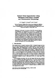
connectivity is 18, while the notation ”6” implies 6-connectivity whose dual connectivity is 26. This distinction is necessary in order to correctly compute topological numbers under 6-connectivity with different dual connectivities. An object X has a handle if and only if there exists a closed n-path in X that can not be compressed to a point through a connected deformation. For example, as shown in Fig. 1a, the closed path abcdef a can be compressed to a point. For an object X, the existence of handles depends on the chosen pairs of connectivities. As shown in Fig. 1a, when n = 6 and n ¯ = 26, there exists ¯ef¯g¯a a handle since the closed 26-path a ¯¯b¯ cd¯ ¯ can not be compressed to a point; when n = 6+ and n ¯ = 18, points a and b are not 18-connected, there exists no handle. In Fig. 1b, it has been illustrated that, when n = 18 or n = 26, the n-closed path abcdef ga can not be compressed to a point, there exists a handle; when n = 6 or n = 6+ , there exists no handle.
(a)
(b)
Fig. 1. Illustration that the existence of a handle depends on the chosen pairs of connectivities
¯ have exactly The foreground object X and its inverse background object X the same number of handles in case a pair of compatible connectivities is used. ¯ where Therefore, the tunnel associated with a handle of X is a handle in X, ¯ there exists a closed n ¯ -path in X that cannot be deformed to a point through connected deformation. The number of handles of an object is called the genus of the object. There are two types of filters which can be used to correct the topology of an input segmentation: foreground filters and background filters. Handles removed by a background filter correspond to tunnels filled in the foreground object. In the algorithm described here, both filters are applied at continuously increasing scales until all topology errors are fixed. Figure 2 shows the idea behind the development of each step. Morphological opening is used as a multiscale analyzer to detect handles at different scales. Figure 2b shows how the opening operation divides the foreground object into two classes. Points in the largest connected component of the opened object are called body points, and points in the residue of the original object and body set are called residue points (Fig. 2c). Thus, the body set consists of one and the residue set of many connected components. This method was designed to transfer as many points as possible from the residue back to the body component. Unfortunately, with complex shapes as in brain segmentations, opening can create ”false” tunnels in the body component. Thus, the body set must be grown without introducing handles, but with filling the ”false” tunnels. This can be done by
402 R1 R2
Opening
Labeling
B
R3
(a)
(b)
(c) Adding nice residues back
Cutting whithin residues
Final result
(f)
R4
(e)
R2
R4
(d)
Fig. 2. Illustration of the basic idea behind the approach [7]
only adding nice points [2] from the residue set. The nice points can be detected like the simple points defined in [6]. Definition 5 (Nice Point) Suppose that we add a point from the background ¯ to the foreground object X. It is a nice point if and only if Tn (x, X) = 1. object X It is equivalent to say that the n-components of X are preserved. The concept of nice points is necessary because morphological opening can introduce tunnels in the body, and these should be filled. Since a simple point ¯ = 1 – and a nice must satisfy two topological criteria – Tn (x, X) = Tn¯ (x, X) point only needs to satisfy one, Tn (x, X) = 1, adding a simple point to the body preserves the topology of the body, but adding a nice point allows a tunnel in the body to be filled. The morphological opening was done by using a distance transform. The distance of a point within the object to its surface is the length of the shortest line to the surface. The chamfer distance transform is a quick way to calculate this distance. The morphological opening sequentially applies morphological eroding and morphological dilating: The erosion with a threshold r removes all points of the object with a distance less than or equal to r. This distance is the scale r. The dilation adds all points of the background with a distance less than or equal to r to the surface after the erosion. If there are regions within a handle which cannot fit a ball of radius r, then the handle can be broken into body and residue parts. For each residue component R, we performed the following iterative procedure: Algorithm 1. Residue Component Expansion (RCE): 1. Recursively add each point of R to the body set B if it is a nice point. If each point of R is added back, then stop; otherwise, go to step 2 (Fig 2d). 2. From R, find the set S of residue points that are adjacent to the body B. 3. Find and label all connected components in the set S. 4. Take the largest connected component L. 5. For each point of L, add it back to B if it is a nice point (Fig. 2d-f). 6. If no points can be added back, stop; otherwise, go to step 2. Note that in steps 2-5, the largest set of border points (if there are nice points) is added to the body. The criterion of nice points ensures that the final
403 Fig. 3. WM/GM surface before and after topology corrections
residue points are not added back to the body and are positioned at the thinnest parts of the handles.
3
Results and discussion
We applied the method to the labeled version of the ICBM single subject MRI anatomical template (www.loni.ucla.edu/ICBM/ICBM BrainTemplate.html). The image size is 304 × 362 × 309 voxels. Cortical gyri, subcortical structures and the cerebellum are assigned a unique label. Processing time for each volume was between 0-7 minutes except the white matter segmentation on an Intel Pentium IV 3.0-GHz CPU. Processing time for the white matter segmentation volume was about 14 minutes. The tessellation of each topologically corrected segmentation has the topology of a sphere, i.e, it has an Euler characteristic of two [2], corresponding to a genus of zero. Fig. 3 shows two sample rendered surfaces before and after topology correction. This algorithm changed between 0.0% and 1.8% of the voxels for each of the segmented volumes of the labeled ICBM atlas, with an average of 0.05%.
References 1. Shattuck D, Leahy M. Automated graph-based analysis and correction of cortical volume topology. IEEE Trans Med Imaging 2001;20(11):1167–1177. 2. Han X, Xu C, Neto U, Prince JL. Topology correction in brain cortex segmentation using a multiscale, graph-based algorithm. IEEE Trans Med Imaging 2002;21(2):109–121. 3. Chen L, Wagenknecht G. Automated topology correction for human brain segmentation. Procs MICCAI 2006;2:316–323. 4. Wood Z, Hoppe H, Desbrun M, Schroeder P. Removing excess topology from isosurfaces. ACM Transactions on Graphics 2004;23:190–208. 5. Kriegeskorte N, Goebel R. An efficient algorithm for topologically correct segmentation of the cortical sheet in anatomical MR volumes. NeuroImage 2001;14:329–346. 6. Bertrand G. Simple points, topological numbers and geodesic neighborhoods in cubic grids. Pattern Recognition Letters 1994;15:1028–1032. 7. Chen L, Wagenknecht G. Topology correction in brain segmentation using a multiscale algorithm. Advances in Medical Engineering, in Proceedings in Physics 2006.