(2) feature-based recognition procedures for cabinets, tables, and other .... resulting point cloud is polygonally reconstructed and object classifying and ...
Towards 3D Object Maps for Autonomous Household Robots Radu Bogdan Rusu, Nico Blodow, Zoltan Marton, Alina Soos, Michael Beetz Intelligent Autonomous Systems, Technische Universit¨at M¨unchen {rusu, blodow, marton, soos, beetz}@cs.tum.edu
Abstract— This paper describes a mapping system that acquires 3D object models of man-made indoor environments such as kitchens. The system segments and geometrically reconstructs cabinets with doors, tables, drawers, and shelves, objects that are important for robots retrieving and manipulating objects in these environments. The system also acquires models of objects of daily use such glasses, plates, and ingredients. The models enable the recognition of the objects in cluttered scenes and the classification of newly encountered objects. Key technical contributions include (1) a robust, accurate, and efficient algorithm for constructing complete object models from 3D point clouds constituting partial object views, (2) feature-based recognition procedures for cabinets, tables, and other task-relevant furniture objects, and (3) automatic inference of object instance and class signatures for objects of daily use that enable robots to reliably recognize the objects in cluttered and real task contexts. We present results from the sensor-based mapping of a real kitchen.
I. I NTRODUCTION Maps (or environment models) are resources that enable robots to better perform their tasks. Using maps robots can better plan their own activities and recognize, interpret, and support the activities of other agents in their environments [1]. Most robot maps acquired and used so far primarily enable robot localization and navigation [2]. With few exceptions, in particular in the area of cognitive mapping [2], [3], but also including [4], [5], maps do not represent objects relevant for other robot tasks. Objects are in most cases geometric primitives such as lines and planes that make maps more compact and abstract [6]. In contrast, robots that are to perform manipulation tasks in human living and working environments need much more comprehensive and informative object models. Consider, for example a household robot that is to set tables. Such a robot must know that cups and plates are stored in cabinets, that cabinets can be opened to retrieve the objects inside, that the visual system cannot see the objects inside a cabinet unless the door is open. It must also know in which cabinets given objects are stored to not have to search for them. In addition, the map should also enable the robot to easily recognize the objects of interest in its work space. Our research agenda aims at investigating the representations, the acquisition, and the use of robot maps that provide robots with these kind of knowledge about objects and thereby enable autonomous service robots, such as household robots, to perform their activities more reliably and efficiently. This paper presents substantial steps towards the realization of such maps and the respective mapping mechanisms.
Conceptually, we perform a feasibility study that demonstrates how robot maps containing (1) object representations for objects such as cabinets, tables, drawers, etc and (2) object libraries for objects of daily use can be represented and acquired. The main technical contributions of this paper are the following ones: (1) a novel robust, accurate, and efficient algorithm for constructing complete object models from 3D point clouds constituting partial object views, (2) featurebased recognition procedures for cabinets, tables, and other task-relevant furniture objects, and (3) automatic inference of object instance and class signatures for objects of daily use that enable robots to reliably recognize the objects in cluttered and real task contexts. The remainder of the paper is organized as follows. The next section introduces our map representation and gives an overview of the mapping process. Section III describes the theoretical algorithms as well as their implementation. Sections IV and V describe the computational mechanisms for acquiring the environment maps and the object libraries respectively, as well as the experimental results obtained. We conclude with a short discussion of related work, our conclusions, and a sketch of our future work. II. E NVIRONMENT M APS AND THEIR ACQUISITION In this section we first conceptualize a kitchen from the view of a household robot that is to perform tasks such as setting the table, preparing meals, and cleaning up. We then describe how we represent this conceptualization as a robot map. We finally consider variants of computational problems for acquiring such robot maps and give an overview of the mapping program we implemented.
Fig. 1.
Point clouds representing objects.
A. Kitchens through the Eyes of Household Robots Looking through the eyes of household robot the kitchen is a room that essentially consists of a set of cabinets, containers with front doors, shelves, which are open containers, and tables — horizontal planes that can be used for performing
kitchen work, having meals, etc. Some of the cabinets have specific roles: the fridge keeps food cold, the oven and microwave is used to cook meals, the dishwasher to clean the dishes after use. There might be more pieces of furniture that have important roles for the robots’ tasks, but for now we only consider these ones. All other types of furniture, such as chairs are uniformly considered to be obstacles. The kitchen also contains smaller objects with changing locations, such as food, ingredients, cooking utensils, and small appliances such as coffee machines. For these objects the robot needs libraries of object representations that can be used to find and recognize these objects, to keep track of their status, etc (see Figure 1). B. Object Maps of Indoor Environments Our map representation is an extension of RG (RegionGateway) maps proposed by Schr¨oter et al. [4]. RG maps are tuples hR; Gi, where R denotes a set of regions and G is a set of gateways that represent the possible transitions between regions. A region has a class label (“office-like” or “hallway-like”), a compact geometric description, a bounding box, one or two main axes, a list of adjacent gateways, and the associated objects O.
The object library contains the small appliances and the objects of daily use, such as ingredients, cups, plates, pots, etc. These objects are moved around and might change their states: cups can be full, empty, used, to be used, clean, etc. These objects are indexed spatially, functionally and as affordances. C. The Mapping Problem In general the mapping problem is to infer the semantic object map that best explains the data acquired during the mapping process. The sensor data is a sequence hvi , posei i where vi is a point cloud where each point has an hx, y, zi coordinate and possibly additional perceptual features associated with it, such as its color. The scans cover the environment to be mapped and each point cloud has sufficiently large overlap with previous scans such that it can be roughly spatially aligned with previous scans. posei specifies the position and orientation of the recording sensor and might be unknown if the robot cannot estimate the position of its sensor. The output consists of a compact obstacle representation of the environment. In addition, the system is to represent the cabinets and drawers that it sensed in their closed as well as opened state as objects with the respective furniture category. The system also has to represent the tables and shelves explicitly and label them respectively. given: { hv1 , pose1 i, ..., hvn , posen i } estimate: a compact and accurate polygonal representation of v1 ∪...∪vn biased towards planar rectangular surfaces infer: object models for cabinets, drawers, shelves, and tables. D. Overview of the Mapping System The operation of the mapping system described in this paper is depicted in Figure 3.
Fig. 2.
Depiction of segmented cupboards in a kitchen.
In this paper we consider how the objects O are represented and how the models of these objects are acquired. The objects O are a tuple hF ; OLi, where F is the set of “furniture-like” objects and OL is the object library. The “furniture-like” objects F is a set of objects that include geometric 3D models, position and orientation, and an object class label. Object classes are cabinets, drawers, shelves, tables, and obstacles, where obstacles are all the objects that do not fall into the first four classes. Cabinets are cuboid containers with a front door that might contain objects of the object library OL. Some cabinets have specific purposes such as the oven, the refrigerator, and the dishwasher. The other cabinets are used to store objects. Tables are another important subclass of furniture-like objects. They are horizontal rectangular flat surfaces approximately at hip height that satisfy some given minimal size and length requirements. Similarly, we have drawers and shelves as additional furniture-like object classes.
Fig. 3.
The architecture of our system.
The first module Acquiring Point Models constructs comprehensive and accurate point models of the individual views provided by the sensor. The point models are then further processed by the type specific mapping components: the Object Modelling and the Environment Mapping module. The object and furniture models returned by these models are
then combined into the Semantic Map. The Acquiring Point Models module first classifies individual point measurements with respect to whether or not they are outliers. Outliers are removed. After outlier removal measurement points are clustered and additional features are extracted to make the consistent integration of different views more efficient and more robust. The integration is done by an iterative optimization algorithm that tries to minimize the distance of points that are believed to correspond to the same 3D points. The details of the algorithm are explained in Section III. The steps Object and Environment Modelling are specific to the aspect of the environment that is mapped. Object Modelling acquires models of the objects of daily use (see Figure 1). Object modelling smoothes object surfaces and reconstructs occluded surfaces through point resampling. The resulting point cloud is polygonally reconstructed and object classifying and identifying features are inferred. Environment Modelling estimates polygonal representations but also recognizes and analyzes large rectangular planes. Special purpose “sensing“ routines look for voxel clouds occluded by rectangular planes — the cabinets, for large horizontal rectangular planes — the tables, shelves, and drawers. The results of both modules are collected into the semantic object map. III. ROBUST ACQUISITION OF P OINT M ODELS The main data structure used by our algorithms is represented by point clouds. The sensors produce several point clouds, each corresponding to a view or snapshot taken by the respective sensor. A point cloud is a set of points, each specifying an hx, y, zi position in space, possibly associated with additional information such as the brightness or the color of the respective point. The workhorse of our object mapping approach is the robust registration-based object reconstruction method. It solves the following model acquisition task: given multiple views of the object to be mapped and possibly an estimation of the sensor position (not mandatory), compute a transformation that can align the views together. The algorithm outputs a polygonal reconstructed model of the object where sensor noise is largely removed based on statistical inferences and missing pieces of surface information are added. The computational problem is difficult for various reasons. Due to the physical limitation of sensors and their limited line of sight, several ”images” from multiple locations must be taken in order to obtain a complete representation of the object. The data is also noisy and often contains a substantial number of outliers. Also many objects of daily use are so complicated that self occlusions cannot be compensated by taking additional recordings. Last but not least, the computations have to be performed on huge data clouds, which prevents the use of straightforward computation techniques. A. Overview of the Robust Acquisition Our object mapping approach satisfies the requirements stated in the last section in that it constitutes a novel
combination of computational ideas being largely independently developed in the research areas of computer graphics, robotics, and scientific computing. We combine methods for building accurate geometrical representations of 3D objects, developed by researchers in the computer graphics community [7], [8] as well as robotics [9], [10] with robust estimation techniques widely used in robotics and computer vision [11]. In order to make the computation processes feasible we apply clustering techniques and techniques from scientific computing to deal with the high volume of data. The basic idea of the algorithm is to construct complete point models by aligning the point clouds of the corresponding object views. This is done by an iterative improvement algorithm that repeatedly rotates and positions a newly acquired point cloud P d , such that it optimally complements another point cloud taken of the same object or scene, which we call the point model Qd . A 50% overlap is however required between the feature points (not the original point sets) as defined by the robustness of the estimator. The fitness function is defined as a distance metric between points in the first scan and the corresponding points in the other scan. This is done by the following computational steps: 1) initialization. • noise removal. The raw data coming from the sensors d is preprocessed and constituting the point cloud Praw using statistical techniques[12] in order to eliminate outliers and reduce noise. d | dist(pdi , pdj ) > µ+dthresh ·σ} (1) P d = {pdi ∈ Praw
Fig. 4. •
Mean distances in a noisy point cloud representing a cup.
computing an initial positioning hypothesis of the point cloud. The point cloud P d is positioned in the neighborhood of the model cloud Qd , such that it lies within the convergence area of the algorithm. For this purpose, the position and orientation estimate of the sensor is used. If the estimate is not available or unreliable, the positioning of P d is done based on normalizations and rotations resulting from its principal components (PCA) using eigenanalysis. n m 0 0 1 X 1X p , q = q − qi p = p − i i i i i n i=0 m i=0 SVD
Cp = P T · P = Up · Sp · VpT (2) SVD T T Cq = Q · Q = Uq · Sq · Vq Where Cp and Cq are the covariance matrices of the de-meaned point sets. The resulting transformation is defined by: T = Qd − (Uq · UpT ) · P d 2) Determining features for optimizing the point cloud alignment. Several geometrical (and visual - where color or intensity data is present) features are extracted and
different level of detail views are generated for the point cloud (see Figure 5).
Fig. 5.
Normal point surface and curvature estimation features.
3) clustering is applied to the point cloud for dimensionality reduction (a cluster is replaced by its center of mass) and faster search operations 4) a robust registration technique is applied to merge multiple views together in order to form a complete model B. Point cloud registration As presented above, the multiple observations gathered from the sensors need to be registered together in order to form a model which characterizes the target object. Several registration methods exist, ranging from those that compute only rigid transformations, to those applicable to deformable surfaces. In our work, we treat all objects of interest as being rigid, thus we are interested in finding out the transformation (rotation and translation) which minimizes the distance error in a least-squares sense. Specifically, we are looking for the transformation: T(P,Q) = {R · P + t | R = [3 × 3], t = [1 × 3]} which minimizes the error e(R,t) =
N 1 X θ||qi − R · pi − t||2 N i=1
where P and Q represent the observation (point clouds), R is a 3x3 matrix representing the rotation, t a 1x3 column vector representing the translation, and θ is a weight of the current evaluated point correspondence. One of the most widely used rigid registration algorithms is the iterative closest point (ICP) [13], [12]. Two big disadvantages of the classical ICP algorithm, besides its speed, make it unappealing for robotics: the wideness of the convergence basin (highly correlated with the needed initial alignment) and the correspondence problem (ICP assumes that each point from the source point cloud has a correspondence in the target point cloud). We propose the use of an ICP-like algorithm which we developed: RnDICP (Robust-nD-ICP - see below). Our approach is twofold: we first process both point clouds in order to extract the most important features that could be used in the registration process (see below). Then, in the actual registration process, we try to include any additional information that we have or can extract from the sensor data, thus boosting the searching dimensionality. This means that, in comparison to the classical ICP which attempts to minimize a 3D mean distance metric between the two point clouds, our algorithm attempts to minimize a nD distance
(eg. 6D for XYZ and RGB color information, 9D for XYZ, RGB and nXnYnZ normal information, etc). The algorithm is summarized as follows: 1) Statistically remove noise and outliers from the P d and Qd point clouds (see Equation 1). 2) Provide an initial guess for the registration algorithm by aligning the point cloud P d as close as possible to the model Qd . If no position and orientation information are available from the sensor, perform eigenanalysis/PCA and use the principal components for rotation (see Equation 2). 3) Estimate geometric primitives and compute features such as surface point normals and curvature flatness metrics, etc (see Figure 5). 4) Cluster the model point cloud Qd into k clusters Ck = {c1 , . . . , ck }. 5) Select the best feature points (minimal subset) from the source point cloud Pfd = {pdi ∈ P d | Fpi > µ + dF · σ} 6) Repeat the following steps until either the number of iterations reaches a given maxIterations value or the registration error drops below a given errValue threshold d • For every selected feature point in cloud Pf , search d for a corresponding point in cloud Q . Qdn = {qnd 1 , . . . , qnd s } v u d uX dist(Pf , Qn ) = mint θ(Pfi , Qin )2 i=1
Statistically remove unlikely matches using the methods presented in [12]. • Compute the rigid transformation T = (R, t) using the singular value decomposition (SVD) of the covariance matrix. d • Apply the transformation to Pf , and adjust the rest of the point attributes (eg. rotate normals). Pfdj = R · Pfj−1 +t d • Compute the registration error metric �. � = M SE(dist(Pfd , Qdn ))) The result of the RnDICP process will be a registered nD model, containing the X,Y,Z point coordinates together with normal information (nX,nY,nZ) as well as extra features (eg. curvature flatness [14]). Where available, R,G,B color information will be included. Among the computed features for registration, we use the ideas presented in [14], where an edge and boundary detection algorithm is performed in order to isolate the important characteristics of the cloud from the rest. The edges of objects can be calculated from the curvature information, as they are characterized by high changes in curvature. This however won’t find the boundary points in the point cloud, as there is no change in curvature for points residing on the outer border of the cloud. Boundary points can be easily identified in 2D, as the maximal angle formed by the vectors towards the neighboring points will be larger for boundary points than for points that are on the inside of an object. In 3D however, such •
angle cannot be computed, still, the method can be applied if one projects a neighborhood on a local reference plane, and transforms the coordinate system to lie on that plane. Mathematically this is the same problem as the detection of peaks in distances when removing outliers. C. Point cloud processing and resampling Because of noise and measurement errors during the scanning process, the model will contain outliers, or even holes, which, if left alone, would disrupt the polygonal reconstruction process. Besides the outliers, which can be detected statistically (see Equation 1), point clouds obtained with laser scanners contain small measurement errors, making a surface look thick. Also, after the registration process, unprecisely aligned surfaces can appear doubled. These anomalies can be smoothed using our proposed Robust Moving Least Squares (RMLS) algorithm. The algorithm is summarized as follows: given a point cloud P d , we want to reproduce the complete smooth surface it represents, by resampling (either upsampling or downsampling) and discarding unwanted data. 1) The coordinates are normalized using the diagonal of the point cloud’s bounding box, ensuring a unity maximal distance between points. We use h = µ+k·σ as our weight factor, where µ is the mean and σ the standard deviation of the mean distances between points 2) An initial guess is computed by approximating the point cloud with a set of points Q3 that are in the vicinity of the original points and their coordinates are integer multiples of a specified resampling step size s: xyz pi xyz 3 3 Q = {qk ∈ R | qk = s · s , pj ∈ P d } The uniqueness of the obtained points must be ensured and extra points must be added to areas where a hole was detected. The algorithm is similar to the one for boundary points detection, with the difference that here we check if a point is inside of an object, so the computed maximal angle must be sufficiently small to ensure correct filling. To ensure that the checked point is close to the surface, its height above the reference plane should be limited with the step size. 3) For each point qk ∈ Q3 to project, a local neighborhood is selected, by using either a fixed number of nearest neighbors, or all neighbors in a fixed radius. The first method can result in neighbors that are relatively far away form the currently fitted point, and their influence must be minimized when fitting the point. Therefore, the weights are assigned to every neighbor pj ∈ P d based on the distance to the currently fitted point (see the equation below). The second method has the disadvantage that it may yield too few neighbors if the search radius is too small, but it ensures that the neighbors will surround the point to be fitted. dist(pxyz ,qk )2 j exp − , h2
qk w(p = qk ∈ Q3 , pj ∈ Pkd j) 4) A local reference plane is selected for coordinate transformation. To fit a plane to the local neighborhood Pkd ,
the minimization of the weighted squares of the error (defined as the sum of weighted distances of the points from the plane) was suggested by an iterative projection approach [15]. This method, although weighted, takes into account the whole neighborhood of the projected point, meaning that it will be influenced by a relatively small patch of outliers, which we found to be common in point clouds obtained by laser scanners. These groups of outliers cannot be eliminated statistically as in Equation 1 because they have approximately the same density as the points that are actually on the surface, so a method with a larger breakdown point is needed. We propose a weighted distance based version of the Random Sample Consensus (RANSAC) algorithm, which will yield good results for up to 50% noise in the neighborhood. d To identify the inliers pl ∈ Pin ⊂ Pkd , a random sample is selected from the neighborhood and a plane D is fitted to them. To measure the probability that the obtained plane is correct, the weighted distances of the points near the plane are summed and mapped on the (0, 1) interval. Iterating through a statistically defined number of steps, the inliers will be obtained as the points close to the fitted plane. These inliers will be used as the reduced neighborhood of the projected point. It must be noted that the weighting ensures that the plane will be fitted to points that are closest to qk . A comparison between the Weighted Least Squares and our Weighted RANSAC can be seen in Figure 6.
Fig. 6.
WLS vs. WRANSAC (dark green) for a cloud with 10% outliers
The fitted plane’s equation and the curvature can be obtained by performing eigenanalysis on the covariance matrix of the selected inliers. The color of the obtained point can be approximated with the weighted average of the inliers’ colors. −1 X q X qk Pg = 1 − w(pkj ) · w(p · D(pj ) j) pj ∈Pkd
pj ∈Pkd D(pj )