Towards Automated Selection of Estimation of Distribution Algorithms Fernando G. Lobo
Cláudio F. Lima
DEEI-FCT, University of Algarve Campus de Gambelas 8005-139 Faro, Portugal
Centre for Plant Integrative Biology School of Biosciences University of Nottingham, UK
[email protected]
[email protected]
ABSTRACT This paper discusses automated selection of estimation of distribution algorithms for problem solving. A specific method inspired in the parameter-less GA is proposed. Other alternatives are also briefly mentioned as promising research directions to address the problem.
Categories and Subject Descriptors I.2.8 [Artificial Intelligence]: Problem Solving, Control Methods, and Search
General Terms Algorithms, Performance
Keywords Estimation of distribution algorithms, Parameter control, Automated selection of EDAs.
1.
INTRODUCTION
As opposed to other evolutionary algorithms (EAs), estimation of distribution algorithms (EDAs) don’t use explicit variation operators such as crossover and mutation. Instead, they learn a probabilistic model from a set of promising solutions, and use the resulting model to predict where other good solutions might be. EDAs are also sometimes referred to as Probabilistic Model-Building Genetic Algorithms (PMBGAs) and have been used efficiently in solving problems where traditional EAs perform poorly [28] [14] [18]. EDAs can be classified into different classes depending on the type of probabilistic models that they can build [24]. The most simple EDAs use univariate models which treat the decision variables of an optimization problem as independent variables [13], [1], [19], [11]. Bivariate EDAs on the other hand allow probabilistic models that can capture pairwise dependencies between variables [5], [2], [27]. Multivariate EDAs are the more complex ones and can capture an
Permission to make digital or hard copies of all or part of this work for personal or classroom use is granted without fee provided that copies are not made or distributed for profit or commercial advantage and that copies bear this notice and the full citation on the first page. To copy otherwise, to republish, to post on servers or to redistribute to lists, requires prior specific permission and/or a fee. GECCO’10, July 7–11, 2010, Portland, Oregon, USA. Copyright 2010 ACM 978-1-4503-0073-5/10/07 ...$10.00.
arbitrary number of dependencies among decision variables [9], [23], [22], [7]. EDAs based on univariate models are the simplest ones and don’t include structural learning. They have been shown to be operationally equivalent to simple GAs with uniform crossover [11]. The more complex EDAs do include structural learning which can be based on learning chain dependencies, tree dependencies, and more general factorizations such as Bayesian Networks or Factor Graphs. These more complex EDAs use Machine Learning techniques to learn the structure of the problem. It is therefore not surprising that these algorithms can outperform traditional EAs that rely on fixed operators, and which may not respect important (unknown) dependencies among a problem’s decision variables. There is a cost, however, when using these EDAs as opposed to simpler evolutionary methods. Learning the structure of the problem is a time consuming operation which is typically done at every generation of the algorithm. (Indeed, a lot of the latest research work in the area of EDAs has been conducted in order to try to enhance the performance of EDAs from that perspective. Examples include paralellization of the model building phase [20], model building relaxation [6], and incremental [7] and sporadic model building [29].) For many problems, the extra effort required by the model-building phase of an EDA can be well worth it. But for other (simpler) problems, it is likely to be unnecessary. Given an optimization problem, the choice of which EDA is the most appropriate for the problem at hand is an interesting question. The general recommendation is to use a univariate EDA for simple problems, a bivariate EDA for somewhat more difficult problems, and a multi-variate EDA for the most difficult ones [21]. The major problem from a practitioner’s point of view is that problem difficulty is difficult to estimate. In a typical scenario the user has no idea of how difficult a problem is, and therefore, no idea of what kind of EDA should be used in the first place. The solution to this dilemma is generally solved by trial and error: Try a univariate EDA first and if not happy with the results, try a bivariate EDA. If still not happy try a multi-variate EDA. To make matters worse, this trial-and-error procedure gets compounded as the performance of a given EDA depends on its parameter settings. In this paper we present some ideas that can be used to automate the trial-and-error way of selecting an EDA for a given problem. The idea is to design a meta algorithm that rationally decides which EDA is best for the problem at hand as the search progresses. This can be achieved by
using techniques similar to those that have been used for adaptation of parameters in evolutionary algorithms [17]. The paper is organized as follows. The next section discusses related research, section 3 presents a method inspired in the parameter-less GA that can be used to automate EDA selection, section 4 briefly mentions other promising research directions, and section 5 summarizes and concludes the paper.
2.
RELATED WORK
This section discusses related research. In particular, we give a brief description of hyper-heuristics, describe recent work by Santana et al. [30] on adaptive EDAs, and review the parameter-less GA technique for automating population size.
2.1
Hyper-Heuristics
Different heuristics may have different strengths and weaknesses, therefore some researches argue that it makes sense to try to combine them in some way in order to get the best features of each individual heuristic. According to Burke et al. [3], “The strength of a heuristic lies in its ability to make good decisions on route to fabricating an excellent solution. Why not, therefore, try to associate each heuristic with the problem conditions under which it flourishes and hence apply different heuristics to different phases of the solution process?” This observation is one of the main reasons that led to the development of hyper-heuristics. A Hyper-heuristic (HH) [3] is a heuristic that operates on a search space of heuristics. In its simplest form, a hyperheuristic is a heuristic to choose among a fixed number of heuristics. It can be seen as a kind of meta-algorithm that operates at different levels. At the lower level there are specialized heuristics tailored to a given application domain. At a higher level there is another heuristic that is concerned with the selection of an appropriate lower-level heuristic as the search takes place. Hyper-heuristics are typically more complex at the high-level than at the low level. For example, it is often the case that the low level heuristics are simple methods specialized for a given problem domain. At the higher level, however, it is common to find meta-heuristics such as Genetic Algorithms, Genetic Programming or Learning Classifier Systems. A more recent trend in hyper-heuristics’ research is concerned with heuristics that generate heuristics. As opposed to methods that automatically select heuristics from a predefined set, this new trend aims at generating new heuristics by combining components of existing heuristics. This new approach has been mainly addressed with Genetic Programming [4]. In either case, the main motivation of the hyper-heuristic approach is to raise the level of generality of optimization methods, allowing them to produce good solutions in a wider range of problem domains. The same motivation is present in our work. By automating EDA selection, we aim at raising the level of generality in which EDAs can be applied, allowing them to produce good solutions across a wide range of domains. The topic of EDA selection shares similarities with the work on hyper-heuristics in the sense that both are meta-algorithms concerned with choosing among different search methods as the optimization takes place.
2.2
Earlier work on Adaptive EDAs
Santana et al. [30] have recently proposed a framework for introducing adaptation in EDAs. The authors recognize that although EDAs are more flexible than regular EAs due their ability to autonomously learn a problem’s structure, the class of probabilistic models is usually fixed for the entire run. They suggest that EDAs could gain additional flexibility by being able to also adapt the class of probabilistic models that they are allowed to learn, as well as adapt to the methods used to learn the probabilistic models as well as the sampling strategies. Santana et al. recognize that many of the things that can be adapted in EAs can be applied directly to EDAs with very little or no change (e.g. adaptation of population size, selection and elitism parameters) and have therefore focused on those things that are specific to EDAs (class of probabilistic model, methods used for learning them and the sampling strategies). They then proposed a generalized EDA that includes different types of probabilistic models, learning and sampling methods. The generalized EDA is shown in Algorithm 1. Algorithm 1 Generalized EDA proposed by Santana et al. (2008) 1: t ← 0. Generate M points randomly. 2: repeat 3: Select a set S of N ≤ M points according to a selection method. 4: Learn an undirected-graph-based representation of the dependencies in S. 5: Using the graph, determine a class of graphical models or approximation strategy to approximate the distribution of points in S. 6: Determine an inference algorithm to be applied in the graphical model. 7: Generate M new points from the model using the inference method. 8: t←t+1 9: until Termination criteria are met. The generalized EDA is allowed to use a different class of probabilistic models at each generation. The choice for the class of models depends on the complexity of the dependencies learned in step 4. For example, if the graph only detects very few dependencies, it may make sense to limit the class to univariate models only. The proposed approach however needs to learn the graph of dependencies at every generation, and that by itself can be a time consuming operation that we would like to avoid, if possible.
2.3
Parameter-less GA
The parameter-less GA introduced by Harik and Lobo [10] was developed with the assumption that solution quality grows monotonously with the population size. Based on that observation, Harik and Lobo suggested a scheme that simulates an unbounded number of populations running in “parallel” with exponentially increasing sizes. Their scheme gives preference to smaller sized populations by allowing them to do more function evaluations than the larger populations. The rationale is that all other things being equal, a smaller sized population should be preferred.
Population size
Generation number 1
2
3
4
5
6
7
8
4
1
2
4
5
8
9
11
12
8
3
6
10
13
16
7
14
Figure 1: The parameter-less GA simulates an unbounded number of populations. In the example, the algorithm’s state contains three populations of size 4, 8, and 16. Notice that smaller populations are allowed to do more generations than larger populations. The numbers inside the rectangles denote the sequence in which the generations are executed by the algorithm.
Initially the algorithm only has one population whose size is a very small number N0 . As time goes by, new populations are spawned and some can be deleted (more about that later). Thus, at any given point in time, the algorithm maintains a collection of populations. The size of each new population is twice as large as the previous last size. The parameter-less GA does have one parameter (although Harik and Lobo fixed its value to 4). That parameter (call it m) tells how much preference the algorithm gives to smaller populations. Specifically, it tells how many generations are done by a population before the next immediate larger population has a chance to do a single generation. An example is helpful to illustrate the mechanism. Figure 1 depicts an example with m = 2. Notice that the number of populations is unbounded. The figure shows the state of the parameter-less GA after 14 iterations. At that point, the algorithm maintains three populations with sizes 4, 8, and 16. Notice how a population of a given size does m = 2 more generations than the next larger population. In the figure, the numbers inside the rectangles denote the sequence in which the generations are executed by the algorithm. The next step of the algorithm (not shown in the figure) would spawn a new population with size 32. This special sequence can be implemented with a m-ary counter as suggested by the original authors [10], and also with a somewhat simpler implementation as suggested by Pelikan and Lin [25]. In addition to maintaining an unbounded collection of populations, the algorithm uses a heuristic to eliminate populations when certain events occur. In particular, when the average fitness of a population is greater than the average fitness of a smaller sized population, the algorithm elimi-
nates the smaller sized one. The rationale for taking this decision is based on the observation that the larger population appears to be performing better than the smaller one, and it is doing so with less computational resources (recall that the algorithm gives preference to smaller populations). Thus, whenever such an event occurs, Harik and Lobo hypothesized that as a strong evidence that the size of the smaller population was not large enough, and the algorithm should not waste any more time with it. By doing so, the algorithm maintains an invariant that the average fitness of the populations are in decreasing order, with smaller sized populations having higher average fitness than larger populations. It has been shown that the worst case time complexity of the parameter-less GA is only within a logarithmic factor with respect with a GA that starts with an optimal fixed population size [26]. Elsewhere, Lima and Lobo proposed the combination of a parameter-less EDA approach with iterated local search in an attempt to get the best of both methods [15]. The motivation of that work is somehow similar to the one that we have in the present paper in the sense that we would like to avoid the cost of model building for those cases where it is unnecessary.
3.
AUTOMATED SELECTION OF EDAS: A METHOD INSPIRED IN THE PARAMETER-LESS GA
The most sophisticated EDAs are very flexible algorithms in the sense that they adapt to the problem at hand by building a probabilistic model that is able to capture the structure of the problem. Nonetheless, there is a cost that needs to be paid by these more complex EDAs when the problem does not require structural learning: The EDA still has to spend a non-negligible amount of time to draw such a conclusion. In a problem with ` decision variables, at least ` ´ all 2` pairwise interactions need to be checked as candidate dependencies. Assuming that the population size N = Ω(`), that amounts to an overall complexity of Ω(`3 ). If possible, we would like to avoid such a cost. One idea to achieve that is to use a technique analogous to the one used by the parameter-less GA.
3.1
Similarities with the parameter-less GA
The problem of automating the population size in genetic algorithms has a strong resemblance with the problem of automating the selection of an appropriate EDA for a given problem. In the case of population sizing, it is reasonable to follow the two major principles introduced by the parameterless GA: 1. Give preference to smaller populations by giving them more function evaluations. 2. Eliminate a population if there’s a strong evidence that it produces worse solutions than a larger sized population. Small populations should get preference because they require less effort than larger ones, and it is desirable that an optimization algorithm reaches a good solution quality with as little effort as possible. Likewise, with respect to automating the selection of an appropriate EDA, it is also reasonable to apply similar principles:
1. Give preference to simpler EDAs. 2. Stop using an EDA if there’s a strong evidence that it produces worse solutions than a more complex EDA. Not knowing what’s the best EDA to use, it is better to give preference to simpler EDAs because they are the ones that require less effort. But it is also important to spend some time with more complex EDAs (just like the parameter-less GA spends some time with larger populations). If at any point in time there’s is a strong evidence that the simpler EDA is inferior to a more complex EDA, then we should stop wasting additional time with the simpler EDA (this is akin to eliminating a population in the parameter-less GA).
3.2
Differences from the parameter-less GA
We can observe a strong resemblance between the parameter-less GA and the method that we are suggesting for automating EDA selection. There is a parallel between population size and EDA class: Preference should be given to simpler EDAs, just like preference should be given to smaller populations in the parameter-less GA. But there’s also a couple of differences between the methods. Specifically, for EDA selection, • The number of EDAs is bounded, the number of populations in the parameter-less GA is not. • Preference has to be given in terms of absolute clock time, not fitness function evaluations. In the parameter-less GA, there is no maximum population size. As long as there is computer memory and as long as the user is not satisfied with the solution quality obtained so far, the algorithm can create larger and larger populations. With respect to EDA selection, the number of EDA classes that we would like to explore is finite, and is a relatively small number. To our minds, it seems reasonable to have three kinds of EDAs: a univariate (such as UMDA or cGA), a bivariate (such as MIMIC or BMDA) and a multi-variate (such as ECGA, BOA, EBNA, or hBOA) 1 . With respect to the second difference, in the parameterless GA giving preference to smaller sized populations is achieved by allowing them to execute more fitness function evaluations than a larger population. That makes sense because fitness function evaluation dominates the overall processing time of a genetic algorithm. In the case of EDAs that may not be the case because the time spent on learning a probabilistic model is not negligible. Therefore, a possible solution to this problem is to give preference to simpler EDAs in terms of absolute clock time. In a concrete implementation, the algorithm could alternate between the EDAs running each one for a little while, and giving more time to simpler EDAs. For example, suppose we have 3 EDAs: univariate, bivariate, multi-variate. The execution of the algorithm would resemble the following loop: 1 Since the time spent on model building in ECGA, BOA, EBNA, and hBOA, is of the same order of magnitude, a good choice of multi-variate EDA seems to be hBOA because it is able to solve more complex problems. An alternative would be to keep two multi-variate EDAs, for example ECGA (which doesn’t allow overlapping variables) and hBOA (which allows overlapping and hierarchical decomposition).
loop run univariate EDA for time α2 · T run bivariate EDA for time α · T run multi-variate EDA for time T end loop where α ≥ 1 is a parameter that tells how much more preference should be given to simpler EDAs. The univariate EDA is allowed to run α more time than a bivariate EDA, and the bivariate EDA is allowed to run α more time than a multi-variate EDA. In practice, the value for T should be large enough to allow the multi-variate EDA to do at least one generation since it is not desirable to let generations half done. Notice that the α ratio for the time allocation can only be kept approximately, but that shouldn’t be a problem.
3.3
Configuration of individual EDAs
We have seen how time can be allocated in order to give preference to simpler EDAs. But what about the configuration of each EDA? The performance of an EDA (or any EA) depends strongly on its parameter settings. For EDAs, the most crucial parameter is the population size. For the other parameters (selection pressure, replacement strategy, and so on) both theoretical and empirical work show that reasonable values can be chosen without affecting the overall time complexity of the algorithm. The population size however is a crucial parameter, and can be responsible for the EDA to be able to properly solve a problem or not. Fortunately, automatically finding a good population size for EDAs is something that has been successfully accomplished by using the parameter-less GA technique itself [16] [25]. In summary, we can run parameter-less versions of the EDAs.
3.4
When to discard an EDA
The final issue that needs to be addressed is how to decide when an EDA should be eliminated. Said differently, what constitutes a strong evidence that a simpler EDA is going to produce worse solutions than a more complex EDA? The criterion that we propose is inspired (again) in the parameterless GA technique: • A given parameter-less EDA should be eliminated if and only if its current best population has an average fitness lower than the average fitness of the best population of a more complex parameter-less EDA. An example should help the reader. Table 1 shows an hypothetical state of the algorithm at a certain timestep. The best performing population of the parameter-less univariate EDA is the population sized 800 and its average fitness is 18. The best performing population of the parameter-less bivariate EDA is the population sized 200 and its average fitness is 17. The best performing population of the parameter-less multi-variate EDA is the population sized 100 and its average fitness is 15. In this example, our criterion for eliminating an EDA doesn’t hold: The best performing population of the various EDAs are in decreasing order of average fitness, with simpler EDAs performing better than more complex EDAs (in the example: 18, 17, 15). Suppose however that the average fitness of the best performing population of the parameter-less bivariate EDA was 19 (instead of 17). In that case, the algorithm should eliminate the parameter-less univariate EDA. The rationale for this decision is analogous to the one used when eliminating populations in the parameter-less GA: The bivariate EDA is
Table 1: An example of the algorithm’s state at a certain timestep. Three parameter-less EDAs are maintained, each one keeps a total running time (in the example α = 1.5). Each EDA maintains a collection of populations, each at its own state of evolution. In this particular example, there’s no evidence that the parameter-less univariate EDA is a bad choice. Its best performing population has an average fitness of 18, better than the average fitness of the best performing populations of the other parameter-less EDAs. (t stands for total clock time spent so far, N stands for population size, G stands for the current generation number, and f¯ is the average fitness of the population.) Algorithm
t
parameter-less univariate EDA
225
parameter-less bivariate EDA
parameter-less multi-variate EDA
150
100
N 800 1600 3200 6400 200 400 800 100 200 400
G 16 8 4 2 8 4 2 8 4 2
f¯ 18 17 14 5 17 16 13 15 13 11
The loop can stop at any time whenever the user decides that the solution quality obtained is good enough. Note also that eventually it may happen that there is only one parameter-less EDA maintained, in which case there’s obviously no need for an EDA selection algorithm.
3.5
Influence of the α parameter The overhead of using the proposed automated approach for EDA selection can be quantified by the ratio of the time taken by the EDA selection algorithm over the time taken by the “ideal” parameter-less EDA. We can easily calculate those ratios for the worst case scenarios (corresponding to the case when EDAs are never eliminated). Below, we present the calculations for the 3 cases: (1) the ideal algorithm is the univariate parameter-less EDA, (2) the ideal algorithm is the bivariate parameter-less EDA, and (3) the ideal algorithm is the multi-variate parameter-less EDA. Table 2 shows the worst case overhead for a few sample values of α. Case 1: Univariate EDA is best Overhead =
1 1 α2 T + αT + T =1+ + 2 α2 T α α
(1)
Case 2: Bivariate EDA is best Overhead =
1 α2 T + αT + T =α+1+ αT α
(2)
Case 3: Multi-variate EDA is best producing better solutions than the univariate EDA, and it is doing so with less processing time; a clear indication that the univariate EDA is not expressive enough to capture the structure of the problem at hand. In summary, what we are proposing is a kind of meta parameter-less technique. At the higher level, an invariant is maintained postulating that the average fitness of the best performing population of each lower level parameterless EDA is kept is decreasing order. A skeleton of the proposed EDA selection algorithm is shown in Algorithm 2. Algorithm 2 A skeleton of the EDA selection algorithm inspired in the parameter-less GA 1: loop 2: run parameter-less univariate EDA for time α2 · T 3: run parameter-less bivariate EDA for time α · T 4: run parameter-less multi-variate EDA for time T 5: eliminate parameter-less EDAs (if necessary) to maintain the invariant that the best performing population of the various parameter-less EDAs are in decreasing order of average fitness. 6: adjust T if necessary 7: end loop The last step in the loop (adjust T ) is necessary to ensure that T is large enough for the parameter-less multi-variate EDA to run at least one generation of its largest population. In practice, each EDA should keep a running count of the total time that has been allocated to it since the beginning of the run, and at every iteration of the loop the exact amount of time allocated to each EDA can be adjusted to maintain the α ratio as close as possible.
Overhead =
α2 T + αT + T = α2 + α + 1 T
(3)
Table 2: Worst case overhead values for α = {1.0, 1.5, 2.0} Worst case overhead case 1 case 2 case 3
α = 1.0 3.00 3.00 3.00
α = 1.5 2.10 3.20 4.75
α = 2.0 1.75 3.50 7.00
In practice, the α parameter can be set based on the user’s perceived idea of problem difficulty. If the user suspects that the problem is hard and requires structural learning, then a value of α close to 1.0 might be an appropriate choice. If on the other hand the user suspects that the problem is easy, then it might make more sense to increase the value of α.
4.
EXTENSIONS
The proposed method inspired in the parameter-less GA is a possible way to address the automated selection of EDAs, but it is by no means the only way to do it. Another promising direction is to explore a mechanism similar to those used for adaptive operator selection (AOS) [31] [8]. The idea would be to use an EDA as if was an operator. Having a fixed set of EDAs (again we could have parameter-less versions), each would be selected with a given probability to run for a certain time period. The selection probabilities would then be adjusted based on the performance of the EDA. Note that in this approach the action of a given EDA
can interfere with the action of another EDA in the future. In other words, the various EDAs would be operating on the same population, whereas in the case of the proposal that we make in section 3 the various EDAs are independent of each other. Another interesting line of work is to include non-EDA search algorithms within the framework. For example, instead of starting with a univariate EDA, it might be wiser to start with a multi-restart hillclimber or an iterated local search method. For many problems these methods are likely to produce good solutions faster than any EDA can do. Likewise, we could include a GA with special purpose operators or a GA together with local search, somewhere in between the parameter-less univariate EDA and the parameter-less bivariate EDA (or between the bivariate and multi-variate EDA). This final observation is supported by the work of Thierens [32] and Hauschild and Pelikan [12] that show that GAs together with special purpose heuristics and/or operators, can sometimes be more efficient than complex EDAs.
5.
SUMMARY AND CONCLUSIONS
This paper stresses the importance of automating the selection of EDAs for problem solving. Although EDAs are more flexible than standard EAs in the sense that the probabilistic models that they learn can exploit a problem’s structure, it is also true that the cost of using complex EDAs may not be worth if the problem that is being solved does not require structural learning. This paper proposed an approach inspired on the parameter-less GA technique. An analogy was made with the problem of automating the population size in EAs, and it was argued that in the absence of knowledge about the difficulty of the problem, the technique that we propose should be capable of discovering the correct EDA for a given problem. The discovery has a cost, just like discovering the ideal population size for an EA also has a cost. The proposed approach needs to be validated with computer simulations, and we plan to do so in the near future.
Acknowledgments This work was sponsored by the Portuguese Foundation for Science and Technology under grant PTDC-EIA-677762006.
6.
REFERENCES
[1] S. Baluja. Population-based incremental learning: A method for integrating genetic search based function optimization and competitive learning. Tech. Rep. No. CMU-CS-94-163, Carnegie Mellon University, Pittsburgh, PA, 1994. [2] S. Baluja and S. Davies. Using optimal dependency-trees for combinatorial optimization: Learning the structure of the search space. In Proceedings of the 14th International Conference on Machine Learning, pages 30–38. Morgan Kaufman, 1997. [3] E. K. Burke, E. Hart, G. Kendall, J. Newall, P. Ross, and S. Schulenburg. Hyper-heuristics: An emerging direction in modern search technology. In F. Glover and G. Kochenberger, editors, Handbook of Meta-Heuristics, pages 457–474. Kluwer, 2003.
[4] E. K. Burke, M. R. Hyde, G. Kendall, G. Ochoa, E. Ozcan, and J. R. Woodward. Exploring hyper-heuristic methodologies with genetic programming. In C. Mumford and L. Jain, editors, Computational Intelligence: Collaboration, Fusion and Emergence, Intelligent Systems Reference Library, pages 177–201. Springer, 2009. [5] J. S. De Bonet, C. L. Isbell, and P. Viola. MIMIC: Finding optima by estimating probability densities. In M. C. Mozer, M. I. Jordan, and T. Petsche, editors, Advances in Neural Information Processing Systems, volume 9, pages 424–430. The MIT Press, Cambridge, 1997. [6] T. S. P. C. Duque, D. E. Goldberg, and K. Sastry. Enhancing the efficiency of the ecga. In G. Rudolph et al., editors, Parallel Problem Solving from Nature PPSN X, 10th International Conference, volume 5199 of Lecture Notes in Computer Science, pages 165–174. Springer, 2008. [7] R. Etxeberria and P. Larra˜ naga. Global optimization using Bayesian networks. In A. A. O. Rodriguez et al., editors, Second Symposium on Artificial Intelligence (CIMAF-99), pages 332–339, Habana, Cuba, 1999. ´ Fialho, L. D. Costa, M. Schoenauer, and M. Sebag. [8] A. Extreme value based adaptive operator selection. In G. Rudolph et al., editors, Parallel Problem Solving from Nature - PPSN X, 10th International Conference, volume 5199 of Lecture Notes in Computer Science, pages 175–184. Springer, 2008. [9] G. R. Harik. Linkage learning via probabilistic modeling in the ECGA. IlliGAL Report No. 99010, Illinois Genetic Algorithms Laboratory, University of Illinois at Urbana-Champaign, Urbana, IL, 1999. [10] G. R. Harik and F. G. Lobo. A parameter-less genetic algorithm. In W. Banzhaf et al., editors, Proceedings of the Genetic and Evolutionary Computation Conference GECCO-99, pages 258–265, San Francisco, CA, 1999. Morgan Kaufmann. [11] G. R. Harik, F. G. Lobo, and D. E. Goldberg. The compact genetic algorithm. In Proceedings of the International Conference on Evolutionary Computation 1998 (ICEC ’98), pages 523–528, Piscataway, NJ, 1998. IEEE Service Center. [12] M. Hauschild and M. Pelikan. Network crossover performance on NK landscapes and deceptive problems. MEDAL Report No. 2010003, Missouri Estimation of Distribution Algorithms Laboratory, University of Missouri-St. Louis St. Louis, MO, 2010. ” [13] A. Juels, S. Baluja, and A. Sinclair. The equilibrium genetic algorithm and the role of crossover, 1993. Unpublished manuscript. [14] P. Larra˜ naga and J. A. Lozano, editors. Estimation of distribution algorithms: a new tool for Evolutionary Computation. Kluwer Academic Publishers, Boston, MA, 2002. [15] C. F. Lima and F. G. Lobo. Parameter-less optimization with the extended compact genetic algorithm and iterated local search. In K. Deb et al., editors, Proceedings of the Genetic and Evolutionary Computation Conference (GECCO-2004), Part I, LNCS 3102, pages 1328–1339. Springer, 2004. [16] F. G. Lobo. The parameter-less genetic algorithm:
[17]
[18]
[19]
[20]
[21]
[22]
[23]
[24]
Rational and automated parameter selection for simplified genetic algorithm operation. PhD thesis, Universidade Nova de Lisboa, Portugal, 2000. Also IlliGAL Report No. 2000030. F. G. Lobo, C. F. Lima, and Z. Michalewicz, editors. Parameter Setting in Evolutionary Algorithms. Springer, 2007. J. A. Lozano, P. Larra˜ naga, I. Inza, and E. Bengoetxea, editors. Towards a New Evolutionary Computation: Advances on Estimation of Distribution Algorithms. Springer, Berlin, Germany, 2006. H. M¨ uhlenbein and G. Paaß. From recombination of genes to the estimation of distributions I. Binary parameters. In H.-M. Voigt et al., editors, Parallel Problem Solving from Nature – PPSN IV, pages 178–187, Berlin, 1996. Kluwer Academic Publishers. J. Ocenasek, E. Cant´ u-Paz, M. Pelikan, and J. Schwarz. Design of parallel estimation of distribution algorithms. In M. Pelikan, K. Sastry, and E. Cant´ u-Paz, editors, Scalable Optimization via Probabilistic Modeling, Studies in Computational Intelligence, pages 187–203. Springer, 2006. M. Pelikan. A tutorial on probabilistic model-building genetic algorithms. In GECCO ’09: Proceedings of the 11th Annual Conference on Genetic and Evolutionary Computation, Companion Material, pages 2879–2906, New York, NY, USA, 2009. ACM Press. M. Pelikan and D. E. Goldberg. Hierarchical problem solving by the Bayesian optimization algorithm. In D. Whitley et al., editors, Proceedings of the Genetic and Evolutionary Computation Conference (GECCO-2000), pages 275–282, Las Vegas, Nevada, 10-12 July 2000. Morgan Kaufmann. M. Pelikan, D. E. Goldberg, and E. Cant´ u-Paz. BOA: The Bayesian Optimization Algorithm. In W. Banzhaf et al., editors, Proceedings of the Genetic and Evolutionary Computation Conference GECCO-99, pages 525–532, San Francisco, CA, 1999. Morgan Kaufmann. M. Pelikan, D. E. Goldberg, and F. Lobo. A survey of optimization by building and using probabilistic models. Computational Optimization and Applications, 21(1):5–20, 2002.
[25] M. Pelikan and T.-K. Lin. Parameter-less hierarchical BOA. In K. Deb et al., editors, Proceedings of the Genetic and Evolutionary Computation Conference (GECCO-2004), Part II, LNCS 3103, pages 24–35. Springer, 2004. [26] M. Pelikan and F. G. Lobo. Parameter-less genetic algorithm: A worst-case time and space complexity analysis. IlliGAL Report No. 99014, University of Illinois at Urbana-Champaign, Illinois Genetic Algorithms Laboratory, Urbana, IL, 1999. [27] M. Pelikan and H. M¨ uhlenbein. The bivariate marginal distribution algorithm. In R. Roy, T. Furuhashi, and P. K. Chawdhry, editors, Advances in Soft Computing – Engineering Design and Manufacturing, pages 531–535. Springer–Verlag, London, 1999. [28] M. Pelikan, K. Sastry, and E. Cant´ u-Paz, editors. Scalable Optimization via Probabilistic Modelling: From Algorithms to Applications. Springer, 2006. [29] M. Pelikan, K. Sastry, and D. E. Goldberg. Sporadic model building for efficiency enhancement of hierarchical boa. In M. Keijzer et al., editors, Proceedings of the ACM SIGEVO Genetic and Evolutionary Computation Conference (GECCO-2006), pages 405–412. ACM Press, 2006. [30] R. Santana, P. Larra˜ naga, and J. A. Lozano. Adaptive estimation of distribution algorithms. In C. Cotta, M. Sevaux, and K. S¨ orensen, editors, Adaptive and Multilevel Metaheuristics, pages 177–197. Springer, 2008. [31] D. Thierens. An adaptive pursuit strategy for allocating operator probabilities. In H.-G. Beyer and U.-M. O’Reilly, editors, Proceedings of the Genetic and Evolutionary Computation Conference GECCO-2005, pages 1539–1546. ACM Press, 2005. [32] D. Thierens. A bivariate probabilistic model-building genetic algorithm for graph bipartitioning. In C. Ryan and M. Keijzer, editors, Proceedings of the Genetic and Evolutionary Computation Conference GECCO-2008, Companion Material, pages 2089–2092. ACM Press, 2008.