Towards Parallel Spatial Query Processing for Big Spatial Data Yunqin Zhong1 2 ∗ , Jizhong Han1 , Tieying Zhang1 2 , Zhenhua Li3 , Jinyun Fang1 , Guihai Chen4 1
Institute of Computing Technology, Chinese Academy of Sciences, Beijing, China 2 Graduate University of Chinese Academy of Sciences, Beijing, China 3 Peking University, Beijing, China 4 Shanghai Jiaotong University, Shanghai, China ∗ Corresponding author, e-mail:
[email protected]
Abstract—In recent years, spatial applications have become more and more important in both scientific research and industry. Spatial query processing is the fundamental functioning component to support spatial applications. However, the stateof-the-art techniques of spatial query processing are facing significant challenges as the data expand and user accesses increase. In this paper we propose and implement a novel scheme (named VegaGiStore) to provide efficient spatial query processing over big spatial data and numerous concurrent user queries. Firstly, a geography-aware approach is proposed to organize spatial data in terms of geographic proximity, and this approach can achieve high aggregate I/O throughput. Secondly, in order to improve data retrieval efficiency, we design a twotier distributed spatial index for efficient pruning of the search space. Thirdly, we propose an “indexing + MapReduce” data processing architecture to improve the computation capability of spatial query. Performance evaluations of the real-deployed VegaGiStore system confirm its effectiveness. Keywords-spatial data management; distributed storage; spatial index; spatial query; spatial applications;
I. I NTRODUCTION In recent years, spatial applications such as Web-based Geographical Information System (WebGIS) and LocationBased Social Networking Services (LBSNS) have become more and more important in both scientific research and industry. Spatial query processing is the fundamental function component to support spatial applications. However, the state-of-the-art techniques of spatial query processing are facing significant challenges as the data expand and user accesses increase [1]. With the development of earth observation technologies, the spatial data are growing exponentially year by year (currently in a petabytes scale), and their categories are becoming more diverse including multi-dimensional geographic data, multi-spectrum remote sensing imageries, high-resolution aerial photographs, and so on. Besides, as spatial applications become more popular, concurrent user accesses to spatial applications are becoming highly intensive. The spatial data objects are generally nested and more complex than basic data types(e.g., string). They are stored as multi-dimensional geometry objects, e.g., points, lines and polygons. Moreover, the spatial query predicates are complex. Typical spatial queries are based not only on the
value of alphanumeric attributes but also on the spatial location, extent and measurements of spatial objects in a reference system. Therefore, spatial query processing over big spatial data requires intensive disk I/O accesses and spatial computation. The state-of-the-art techniques of spatial query processing mainly include SDB (spatial database) [2] and KVS (keyvalue stores). SDB provides spatial query language (i.e. spatial SQL) [3], and performs well when handling relatively small spatial datasets in megabytes or gigabytes [4]. However, since spatial queries are usually both I/O intensive and computing intensive, e.g., a single query may take minutes or even hours in SDB [5], the I/O and computation capabilities of SDB can hardly meet the high performance requirement of spatial queries over big spatial data. The emerging KVS systems, such as Bigtable [6], HBase [7] and Cassandra [8], are proved to be feasible alternatives to store big semistructured data for its scalability. They has been adopted in some I/O intensive applications, e.g., Bigtable has been used to store satellite imagery for Google Earth [6]. However, the data in key-value stores are organized regardless of geographic proximity, and they are indexed by key-based structure (e.g., B+ tree) rather than spatial index. Therefore, KVS cannot process spatial queries efficiently. Driven by the above problems, in this paper we propose and implement a novel scheme (named VegaGiStore) to provide efficient spatial query processing over big spatial data and numerous concurrent user queries. Firstly and most importantly, we propose a geography-aware data organization approach to achieve high aggregate I/O throughput. The big spatial data are partitioned into blocks according to the geographic space and block size threshold 1 , and these blocks are uniformly distributed on cluster nodes. Then the geographically adjacent spatial objects are stored sequentially in terms of space filling curve which could preserve the geographic proximity of spatial objects. In practical spatial applications, most clients only focus on a relatively small area and query for adjacent spatial objects within the area. Thereby concurrent clients can be served in parallel by 1 The block size threshold is the maximum size of a block. The partitioning process does not finish until the total size of spatial objects within a partitioned region is smaller than the threshold.
different cluster nodes and adjacent spatial objects can be streamed to clients sequentially without random I/O seeks. Secondly, in order to improve data retrieval efficiency, we design a two-tier distributed spatial index for efficient pruning of the search space. The index consists of Quadtreebased [9] global index and Hilbert-ordering local index, where the global index is used to find data blocks and local index is used to locate spatial objects. Thirdly, we propose an “indexing + MapReduce” data processing architecture to improve the spatial query computation capability. This architecture takes advantage of dataparallel processing techniques to provide both intra-query parallelism and inter-query parallelism, and thus can reduce individual spatial query execution time and afford a large number of concurrent spatial queries. We have implemented VegaGiStore on top of Hadoop [10], an emerging open-sourced cloud platform. VegaGiStore can support numerous concurrent spatial queries for various spatial applications like Web Mapping Services (WMS), Web Feature Services (WFS) and Web Coverage Service (WCS) [1]. Compared with the traditional methods, VegaGiStore improves the average speed-up ratio by 70.98% − 75.89% when processing spatial queries on a 17node cluster, and its average spatial query performance is increased by about 10.3−13.5 times better than that of singlenode spatial databases. Moreover, its average I/O throughput is improved by 99%−235% than that of compared key-value stores. In summation, our contributions in this paper can be summarized as follows: 1) We present a feasible scheme for efficient processing of spatial queries over big spatial data. We tackle the problem through three significant approaches: geographical-aware organization approach for high I/O throughput; two-tier distributed spatial index for data retrieval efficiency; “indexing + MapReduce” spatial querying architecture for parallel processing. Our scheme can be easily integrated into a cloud computing platform (e.g., Hadoop [10]) to support parallel spatial query processing. 2) We have implemented a spatial data management system termed VegaGiStore on top of HDFS (Hadoop Distributed File System) [11] and MapReduce framework [12]. VegaGiStore provides multifunctional spatial queries which most key-value store systems do not have, and it is transparent to spatial applications. Besides, the system evaluations show that VegaGiStore outperforms spatial databases and emerging key-value stores while processing concurrent spatial queries from numerous clients in practical spatial applications. The rest of the paper is organized as follows. Section II details the parallel spatial query processing scheme. Section III presents the performance evaluation. Section IV reviews the related work. Finally, Section V concludes this paper.
II. PARALLEL S PATIAL Q UERY P ROCESSING S CHEME A. Geography-aware Spatial Data Organization Approach 1) Spatial Data Partitioning: We propose a geographyaware quadripartition method to partition a large map layer. The scheme is designed to guarantee that data within a partitioned region are stored on one node, and all spatial data are distributed across cluster according to geographical space. Spatial data objects are logically or physically organized in multi-scale map layers. Spatial object has three attributes: ID(identifier), MBR(Minimum Bounding Rectangle) and object value. A map layer also has three attributes: unique name, MBR and resolution. MBR is an expression of the maximum extents of a 2-dimensional spatial object. MBR is frequently used as an indication of the general position of spatial object, and it is used as spatial metadata for first-approximation spatial query and spatial indexing purpose. Therefore, Spatial applications could access spatial data within different regions from different nodes to provide spatial information services for numerous users. Input: Region(i.e., MBR of map layer) Output: Partitioned Subregions 1: Initiate(region) 2: M SIZE ← 64M B 3: {0, 1, 2, 3} ← {N W, N E, SE, SW } 4: Boolean isValid ← Verify(region) 5: if isValid then 6: for i=0 to 3 do 7: subregion[i] ← Partition(region) 8: end for 9: else 10: exit(0) 11: end if 12: for i=0 to 3 do 13: Verify_Partition(subregion[i]) 14: end for Figure 1.
Verify_Partition(region). Procedure of partitioning a region
The partitioning process is described as follows, and the respective pseudo code is shown in Fig.1. 1) Input and Initialization Process. Input a map layer/region and compute the size of objects including the real data size and additional indices size. 2) Verification Process. If the region size is larger than threshold M SIZE, then set isValid flag to “TRUE”, and go to Step 3; else the region size is not smaller than M SIZE, set isValid to “FALSE” to indicate that it need not to be partitioned. 3) Partition Process. Partitioning the region into four quadrants according to its MBR, and each quadrant represents one subregion. 4) Computing the size of four subregions respectively, and go to Step 2 to verify each subregion recursively and determine whether the subregion should be further partitioned or not. 5) The partitioned process will be executed recursively until all subregions are not larger than M SIZE.
6) If all partitioned regions satisfied valid requirements, return “0”; else terminate the partition procedure. According to the principle of geographic proximity, spatial objects within a region are combined into one data block, so the threshold size M SIZE should be set as large as the HDFS block size in order to guarantee spatial data within a region are stored on the same node, typically set to 64MB, and it can be varied according to dataset amounts and cluster scale. Otherwise, the spatial data within a region may be stored on more than one node, which will reduce data retrieval performance. According to the partition procedure, three deductions are described as follows. • Let κ denote the size of square region, and there are 2κ × 2κ spatial objects in the region whose size is κ. • The upper-left point is defined as the first object of region. • The first κ bits of coordinate(x,y) of the first object are “0”, i.e., x = xn · · · xκ 00 · · · 0 and y = yn · · · yκ 00 · · · 0, where n denotes size of the parent region. The higher (n − κ) bits of coordinates of objects within the region are identical, which is defined as region code, i.e., region code is represented as (yn xn )(yn−1 xn−1 ) · · · (yκ xκ ). Fig.2 shows an example of partitioning a region by quadripartition scheme. The region size κ = 4, its subregions are represented by solid line squares, it contains 24 × 24 = 256 spatial objects which represented by dotted square. 00
01
00
01
02
03
1 02
1
03 300 301
31 302 303
2
2 32
Figure 2.
33
Quadripartition
32
Figure 3.
33
Hilbert-order storage.
2) SOFile: We design a spatial objects placement structure termed SOFile(Spatial Object File). The SOFile is created during partitioned process, and the spatial objects within a subregion are stored in a SOFile named by the subregion’s GC value. Moreover, the raster data are stored as tile objects in SOFile, whereas the vector data are stored as WKB(WellKnown Binary) objects. Taking geographic proximity into consideration, the geographically adjacent objects should stored in sequential disk pages. Spatial objects within a partitioned subregion are stored into the SOFile by space filling curve, and they are organized in Hilbert order instead of Row-wise order or Z order because it has better localitypreserving property [1].
Reserved bits(4B) offset of 1st tile(4B)
X-value of 1st tile(4B) length of 1st tile(4B)
offset of rest tilesĂ
length of rest tiles Ă
Y-value of 1st tile(4B) K-value of region(4B) offset of 2nd tile(4B) length of 2nd tile(4B) offset of 2k *2k tile(4B) len of 2k *2k tile(4B)
real data of 1st tile
real data of 2nd tile
data of rest tiles Ă
data of the 2k *2k tile
Local Index Data
Figure 4. Structure of SOFile for raster data model. SOFileRaster is designed for raster data placement, which contains local indices header and raster objects.
Each SOFile consists of geographically adjacent spatial objects within a specific subregion, and one SOFile occupies one data block. Since there are two conventional spatial data models in spatial applications, we have design two different structures of SOFile for raster tiles and vector geometry objects, respectively. The structure of SOFile for raster data model is shown in Fig.4, which is called SOFileRaster. Moreover, Fig.5 shows the structure of SOFile(termed SOFileVector) for vector data model. MBR of region(16B)
HC of 1st WKBobject(4B) GC value of region(4B)
K-value of region(4B)
offset of 1st WKBobject(4B) length of 1st WKBobject(4B) offset of 2ndWKBobject(4B) length of2ndWKBobject(4B)
offset of rest objectsĂ
length of rest objects Ă
offset of 2k *2kobject(4B) len of 2k *2k object(4B)
1st WKBobject data
2nd WKBobject data
data of rest objects Ă
data of the 2k *2k objects
Local Index Data
Figure 5. Structure of SOFile for vector data model. SOFileVector is designed for vector geometry object placement, which contains local indices header and WKB objects.
Both SOFileRaster and SOFileVector are inherited from SOFile structure, which includes local index header and real data part. Since the raster data and vector data have different function for spatial queries, we design different index structure for the two spatial data models. The local index header is the main distinction between SOFileRaster and SOFileVector, which will be described in SectionII-B2. The local index header contains meta data information of block and index items of spatial objects; the data content part contains real data of spatial objects within the region. Moreover, the size of SOFile is the sum length of indices and real data part. The spatial objects are organized in Hilbert order and assigned unique HC(Hilbert Code), and adjacent spatial objects are stored on sequential disk pages so that it can guarantee geographic proximity and storage locality. Fig.3 shows an example that spatial objects within region R31 are stored in Hilbert order. The leaf node of global index tree is pointed to a data block file whose suffix is “.sof”(spatial object file) on HDFS, and the non-leaf node represents a region that should be partitioned into four smaller subregions for its size is larger than threshold M SIZE. Fig.6 shows an example of hierarchical directory structure details of region(κ = 4) stored on HDFS, which is corresponding to quadripartition schematic shown in Fig.2. The ellipse represents storage directory corresponding to non-leaf node, and rectangle represents data block file corresponding to leaf node. HDFS creates one block for each file, and file blocks are distributed
NameSpace in NameNode
where s and κ denote the size of region and its subregions, (x, y) denotes the coordinates of objects, and ci ∈ {0, 1, 2, 3}.
Global Code 1.sof
0 00.sof
01.sof
02.sof
metadata of 300.sof.meta blk_xxx: DataNode1,DataNode M
30
03.sof 300.sof
DataNode 1
DataNode 2
blk_xxx Index Data
blk_bbb Index Data
ĂĂ
ĂĂ
blk_aaa Index Data
blk_ccc Index Data
Figure 6.
2.sof
301.sof
Other DataNodesĂ
blk_sss Index Data
ĂĂ blk_*** Index Data
GC =
3 31.sof 302.sof
32.sof
s ∑
(2yκ + xκ ) × 4s−κ
(1)
κ=1
33.sof
303.sof
DataNode M
DataNode N
blk_ccc Index Data
blk_bbb Index Data
ĂĂ
ĂĂ
blk_xxx Index Data
blk_aaa Index Data
Hierarchical structure for spatial data on HDFS(κ = 4)
across cluster nodes for load balancing. As shown in Fig.6, the directory hierarchy is quadtree-like structure, the root node of quadtree represents the root directory identified by “Global Code”, and its four children nodes represent subdirectories and “.sof” files. B. Two-tier Distributed Spatial Index The VegaGiStore system must be able to retrieve from a large collection of objects in some space those lying within a particular area without scanning the whole datasets, so the spatial index is mandatory. In order to improve spatial data access performance and optimize spatial queries, we propose a scalable distributed spatial index to accelerate positioning spatial objects on HDFS. Considering geographic proximity and storage locality, the geographically adjacent data should be stored into the same node. Our proposed distributed spatial index is a two-tier scalable index including global index and local index. There are two salient features of the spatial index. The global index is based on the revised distributed quadtree index [13], which is used to determine the data block location. The local index is built by space filling curve and is used to locate spatial objects within a block. Moreover, the distributed index is designed and tuned for spatial applications, which is oriented to improve spatial data retrieval efficiency on HDFS. 1) Global Index: The global quadtree index is created during quadripartition process. The large map layer is partitioned into four quadrants recursively until all subregions are satisfied the threshold. Meanwhile, all spatial objects belong to the map layer is partitioned according to their geographical space, and adjacent objects are sequentially stored into a SOFile. Once a large map layer is split into several subregions, the spatial data are partitioned into many data blocks and uniformly spread across HDFS DataNodes. The global index is quadtree-based, and the global tree structure is represented by Global Code (GC). GC is quaternary code, where GC = c1 c2 , · · · , cs = y1 x1 y2 x2 , · · · , ys xs . GC value can be computed by (1),
According to (1), each region has an unique GC value used to construct global index. As shown in Fig.2, the quaternary numerics denote GC values of regions, e.g., region R300 = 303, R301 = 301, we can derive that the GC value of their parent node is 30. Since the non-leaf node of global index tree only pointed by its GC value, the size of global tree is very small and the global index is resident in memory during retrieval process. Besides, pairs of regions are maintained in the HashMap structure, which are used to obtain MBR information for further spatial query computation. 2) Local Index: The local index is created when subregion data is written into SOFile, and indices data are stored in the SOFile as well. Therefore, the leaf nodes of global quadtree are pointed to the header of spatial object file. The local index is used for indexing spatial objects within SOFile, and the local index header is illustrated as follows. • Metadata information. For the SOFile structure, the first word is reserved for data version; the second and third words are (x, y) coordinate of 1st object; the fourth word is the κ value of the region; the region is determined by its κ value and coordinate(x,y) of the first tile object while processing raster data. For the SOFileVector structure, the first four words are MBR(Minimum Bounding Rectangle) information of the region represented by four double values; the fifth word is HC(Hilbert Code) value of the first WKBobject; the sixth and the seventh word is GC value and κ value of region, respectively. • Index item. The index item contains two fields: offset and length. It means that local index of each spatial object is corresponding to a pair, and the index items of spatial objects are written into block sequentially. κ κ • Indices length. There are 2 × 2 objects, and index length of object is 8 bytes, so the total length of file indices is 22κ+3 bytes. Thus the index length of SOFileRaster and SOFileVector is (22κ+3 + 12) bytes and (22κ+3 + 24) bytes, respectively. C. “Indexing+MapReduce” Data Processing Architecture We propose an “indexing + MapReduce" data processing architecture to improve the spatial query computation capability of VegaGiStore. This architecture takes advantage of data-parallel processing techniques to provide both intraquery parallelism and inter-query parallelism, and thereby can reduce individual spatial query execution time and
provide a large number of concurrent spatial queries. Our scheme is specific to spatial queries including spatial selection, spatial join and nearest neighbors, and the spatial queries are processing in multiple phases. The first filter phase prunes non-qualified objects with spatial index to obtain candidate intermediate sets, and then the qualified candidate objects are transferred as the input of refinement phase. Finally the spatial relation computation examines the actual object representation to determine the query results. 1) MapReduce-based Spatial Query Operator: In VegaGiStore, we have implemented several spatial query operators using the map/reduce paradigm. The spatial query operators are classified into three categories: spatial selection, spatial join and NN(Nearest Neighbor). Moreover, the spatial selection queries contain point query, range query and region query, where the region query includes rectangle query, circle query and polygon query. Besides, the NN query consists of k-NN(k-Nearest Neighbor). In addition, the spatial query algorithms are encapsulated into spatial query operators, and these operators are packaged as map/reduce spatial query library. Therefore, an arbitrary complex spatial query can be implemented by a combination of these query operators. 2) Parallel Execution of Spatial Query: Our scheme takes advantage of data-parallel processing techniques so that it could provide both inter-query parallelism and intra-query parallelism. The inter-query parallelism is obtained by parallel executing multiple spatial queries as independent jobs so that it can support a large number of concurrent clients. The intra-query parallelism can be obtained by parallel execution of two independent phases within an individual spatial query. As shown in Fig.7, the spatial query are processing in two phases, which includes filter phase and the refinement phase. The filter phase searches the global index and obtains the candidate SOFile sets, and these candidates are parallel processed by a map-reduce job at the refinement phase. The details of spatial query execution in VegaGiStore are described as follows. Firstly, the filter operation prunes non-qualified spatial objects simultaneously by searching the global index, and returns the candidate SOFile sets. Since the global index is kept in memory and retrieved by GC(Global Code) of global quadtree, the filter phase will be finished in several milliseconds. The outputs of this phase are GC values of SOFiles that matches the query requirements, and the candidate SOFile sets are used as the input of next refinement phase for further computation. Secondly, the candidate SOFile sets are interpreted into pairs and processed by a map-reduce job at the refinement phase. Since the map-reduce framework relies on the InputSplit and RecordReader, we implement SOFileInputSplit and SOFileRecordReader to generate pairs for Mapper. The map and reduce procedures are described as follows. • Map task. The generated pairs are
•
transferred to SpatialQueryMapper and they are parallel processed by TaskTrackers on the cluster nodes. This process obtains the pairs that satisfying the query conditions. Reduce task. the satisfied pairs are transferred to Reducer. SpatialQueryReducer executes the complex spatial relationship computation for the final query results.
Filter phase
Global Index
Local Index SOFile
Local Index SOFile
Local Index SOFile
SOFileInputSplit
SOFileInputSplit
SOFileInputSplit
SOFileRecordReader
SOFileRecordReader
SOFileRecordReader
SpatialQueryMapper
SpatialQueryMapper
SpatialQueryMapper
Refinement phase
SpatialQueryReducer
SpatialQueryReducer
Query Results
Figure 7. Spatial query processing architecture of VegaGiStore. The filter phase searches the global index and outputs candidate SOFile sets; then these candidate sets are processed in parallel by a map-reduce job at the refinement phase.
Since complex spatial query can be combined by several spatial query operators, and these operators are map-reduce based, the complex spatial query can be executed in parallel on many nodes. Besides, a large number of concurrent spatial queries can be executed simultaneously. Therefore, VegaGiStore could achieve high throughput performance for spatial query processing over big spatial data. III. P ERFORMANCE E VALUATION A. Experiment Environment Our experiments are conducted on a cluster of 17 commodity servers that spread across two racks(i.e., RACK1 & RACK2). RACK1 consists of 8 nodes, and each node has two quad-core intel CPU 2.13GHZ, 4GB DDR3 RAM, 15000r/min SAS 300GB hard disk. RACK2 consists of 9 nodes and each node has a Intel Pentium 4 CPU 2.8GHz, 2GB DDR2 RAN, 7200r/min SATA 80GB hard disk. All nodes are connected through Gigabit Ethernet switchers. Software configurations are detailed as follows. All nodes have identical CentOS 5.5 server edition (kernel 2.6.18), Linux Ext3 and JDK-1.6.0_20. PostgreSQL-9.0.5 cluster, bare Hadoop-0.20.2, Cassandra-0.7.6, HBase-0.20.6 and VegaGiStore are deployed on the cluster. Moreover, Zookeeper-3.3.3 is deployed on 7 nodes to maintain configuration information and distributed synchronization. Besides, we also deploy two spatial databases in RACK1, i.e., commercial Oracle Spatial + Oracle database cluster and open-sourced PostGIS + PostgreSQL cluster.
B. Test Items and Datasets As already mentioned, spatial queries should process large amounts of spatial data, and the spatial query efficiency is heavily depended on both I/O and spatial computation performance, hence we evaluate spatial query performance in terms of two categories, including I/O metrics and spatial query metrics. We evaluate the I/O performance by three frequently-used I/O operations in spatial applications, which includes random reads, sequential reads and bulk loading. Besides, the spatial query efficiency is evaluated by conventional operations, including spatial selection query, spatial join and k-NN query. The real spatial dataset is about 1.379TB and consists of raster and vector datasets, which covers eight map scales with highest resolution is 1 : 5000. The raster dataset contains about 128, 323, 657 file-based tiles, and each tile ranges from several bytes to tens of KBs. The vector dataset consists of geometry objects: (a) TLP contains 314, 851, 774 point objects; (b) TLL contains 81, 991, 436 line objects; (c) HYP contains 16, 749, 181 polygon objects. C. Reads Operations We evaluate two reads operations: random reads and sequential reads, which are used in different application scenarios. Random reads operation is often used for random access of spatial objects within a small region, e.g., reading the spatial object of given location ; sequential reads operation is used to sequentially access adjacent spatial objects within a map layer, e.g., reading all geometry objects within specific map layer. Let R(lon, lat) denote that reading (lon × lat) spatial objects within region R, e.g., R(1, 1) means reading one object, and R(80, 80) means reading 6400 spatial objects. We conduct six groups of comparative experiments for random reads and sequential reads, respectively. The comparisons are VegaGiStore and four other typical systems, including PostgreSQL cluster, bare HDFS, Cassandra and HBase. 1) Random Reads Operation: The random reads performance is evaluated by reading spatial objects with size from R(1, 1) to R(8, 8). As shown in Fig.8, the average random reads performance of VegaGiStore is increased by about 79%, 338%, 96%, 89% than that of PostgreSQL cluster, bare HDFS, Cassandra and HBase, respectively. Since bare HDFS is only tuned for streaming large files, it performs worst while randomly reading small spatial objects. PostgreSQL cluster performs better than key-value stores because it has spatial index. Moreover, VegaGiStore performs even better while randomly reading more spatial objects, e.g., VegaGiStore costs 1.01ms and 20.86ms to reading 1 object and 64 objects, whereas the respective time is 1.12ms and 38.45ms for PostgreSQL cluster. VegaGiStore gains excellent random reads performance due to its geographyaware data organization scheme, and hence it could provide
Figure 8.
Random reads performance.
low latency random access for spatial applications involving a large number of concurrent reads. 2) Sequential Reads Operation: We also conduct six groups of test with size from R(20, 20) to R(80, 80) for sequential reads evaluation, and then each test case is repeated for 10 times, finally collect the average results.
Figure 9.
Sequential reads performance.
As shown in Fig.9, the average sequential reads performance of VegaGiStore is about 198%, 856%, 336%, 309% better than that of PostgreSQL cluster, bare HDFS, Cassandra and HBase, respectively. Moreover, the VegaGiStore performs better when reading more geographically adjacent spatial objects, e.g., it cost only 112ms when reading 6400 spatial objects from VegaGiStore, yet the respective time is 523ms, 1187ms, 593ms and 583ms for PostgreSQL cluster, bare HDFS, Cassandra and HBase. VegaGiStore outperforms compared systems in reads micro-benchmarks because it benefits from geography-aware data organization scheme. VegaGiStore organizes the geographically adjacent spatial objects into sequential disk pages, and hence the objects are successively streaming to clients once seeks to the right position. Moreover, VegaGiStore can support a large number of concurrent reads across multiple nodes because it preserves geographic proximity
and storage locality. Due to ignorance of geographic proximity and absence of spatial index on HDFS, Cassandra and HBase, they may access too many data blocks across multiple nodes while reading geographically adjacent objects, which leads to low sequential reads efficiency. D. Bulk Loading Operation Since most spatial applications are write once read many access model [14], the large amounts of spatial data should be quickly imported into storage systems for rapid deployment of spatial information services. Bulk loading operation is often used for batch import of spatial data in practical spatial applications, e.g., loading multi-scale spatial data across multiple map layers into storage system. We have imported three groups of datasets into VegaGiStore and compared systems respectively, including Linux Ext3(LocalFS), PostgreSQL cluster, bare HDFS, Cassandra and HBase. There are two replicas in all systems and the HDFS block size is set to 64MB. The three group datasets include raster data and vector data, and they are classified as small(64 GB), medium(512 GB) and large(1024 GB) groups.
Figure 10.
I/O throughput and has obvious advantages while bulk loading big spatial data. E. Spatial Query Performance Since key-value stores don’t provide spatial query functions, we compare the spatial queries between VegaGiStore with two typical spatial databases, i.e.,Postgre+PostGIS and Oracle Spatial. The datasets are imported into the three compared systems, and the spatial indices of spatial objects are created as well. Moreover, we have shown the scalability of VegaGiStore on different number of nodes, i.e., VegaGiStore is evaluated on cluster of 1, 2, 3, 5, 7, 9, 11, 13, 15, 17 nodes respectively. Besides, each node runs two map tasks and one reduce tasks in VegaGiStore while executing map-reduce based spatial query jobs. 1) Spatial Selection Performance: We have conducted three groups of experiments(RQ1, RQ2 and RQ3) to evaluate the spatial selection performance. First, we create a rectangular region R with its size is 46.53% of the MBR of HYP dataset; then spatial selection operations is executed in compared systems to find all the objects of vector datasets that geometrically interact with R; finally compute and print the outputs, i.e., the satisfied geometry objects information.
Bulk loading performance.
As shown in Fig.10, the bulk loading time of compared systems is varied with dataset size, and VegaGiStore outperforms other systems in all test cases. Since there are lots of small tiles and geometry objects, the localFS and bare HDFS perform not as well as the other four systems. The bulk loading performance of VegaGiStore gets even better while storing larger dataset. For the small group, the bulk loading time of VegaGiStore is about 17.6 minutes, which is 680%, 510%, 597%, 99%, 235% faster than that of LocalFS, PostgreSQL cluster, bare HDFS, Cassandra and HBase, respectively. On the other hand, it cost about 261.9 minutes for loading large(1024GB) dataset into VegaGiStore, which is about 10.9, 5.13, 6.88, 1.1, 1.36 times faster than compared systems, respectively. Besides, the average I/O throughput of VegaGiStore is about 65.8MB/s, whereas the I/O throughput of LocalFS, PostgreSQL cluster, HDFS, Cassandra and HBase is about 6.9, 11.3, 8.9, 32.9, 27.3 MB/s, respectively. Therefore, VegaGiStore achieves highest
Figure 11.
RQ1 finds point objects of TLP within R.
The spatial selection operation RQ1 is to query all points objects of dataset TLP that within region R. As shown in Fig.11, when processing RQ1 on 2 to 17 nodes, the execution time of VegaGiStore is reduces from 159.09s to 12.71s, whereas the execution time of PostGIS and Oracle Spatial is 168.72s − 76.32s and 152.21s − 69.93s, respectively. The average speedup ratio of VegaGiStore is about 75.32%. Moreover, it should be pointed out that the execution time of VegaGiStore is longer than that of SDB on single node. That is because VegaGiStore depends on MapReduce runtime system, and the MapReduce startup is a costly process. The spatial selection operation RQ2 is to query all lines objects of dataset TLL that within or intersect with region R. As shown in Fig.12, the average speedup ratio of VegaGiStore is about 72.87%, and the execution time is
predicate {(r, s)|r Intersect s, r ∈ S1, s ∈ S2}.
Figure 12.
RQ2 finds line objects of TLL interact with R.
reduced from 308.67s to 27.06s, whereas the execution time of PostGIS and Oracle Spatial is 353.78s − 236.67s and 343.61s − 226.39s with number of nodes increased from 2 to 17, respectively.
Figure 13.
Figure 14.
Spatial join query evaluation.
As shown in Fig.14, the spatial join query performance of VegaGiStore is much better than that of PostGIS and Oracle Spatial. The execution time of VegaGiStore, PostGIS and Oracle Spatial on one node is 1458.39s, 1423.76s and 1396.58s, respectively. However, the execution time of VegaGiStore is reduced obviously as the cluster scales, e.g., the time is 91.37 s with 17 nodes, whereas the respective time is 588.69s and 538.69s for PostGIS and Oracle Spatial. The average speedup ratio of VegaGiStore is about 70.98% when processing intersection spatial join query. VegaGiStore performs better with more nodes, thus it could efficiently process spatial join query involving large datasets. 3) kNN Performance: The kNN query predicate is to find k objects in TLP dataset that are closet to a query point p.
RQ3 finds polygon objects of HYP interact with R.
The spatial selection operation RQ3 is to query all polygons objects of dataset HYP that interact within or overlap with region R. As shown in Fig.13, with RQ3 is processed on 2 node to 17 nodes, the execution time of VegaGiStore is reduced from 752.89s to 55.37s, whereas the execution time of PostGIS and Oracle Spatial reduces not so obviously, i.e., 812.37s − 608.91s and 762.37s − 508.91s, respectively. Besides, the average speedup ratio of VegaGiStore is about 75.89%.Therefore, VegaGiStore achieves distinguished spatial selection performance and has good scalability. 2) Spatial Join Performance: Spatial join query combines objects from two datasets by geometric attributes which satisfy spatial predicate. We conduct experiment to evaluate the spatial join query, where the spatial predicate is intersection. Moreover, the intersection join query is processed over dataset TLL(lines objects), and it answers query such as finding roads across rivers in specific area. We select two spatial datasets S1 and S2 with their size is 30% of TLL. The spatial join performance is evaluated by intersection join operation, i.e., finding objects that satisfy
Figure 15. kNN spatial query performance of different systems(k = 1, 10).
We evaluate the kNN spatial query between VegaGiStore and spatial databases (i.e., PostGIS and Oracle Spatial) where k = 1 and 10. As shown in Fig.15, VegaGiStore outperforms spatial databases running on more than two nodes, and its execution time is reduced from 620.98s to 58.17s with nodes increased from 2 to 17, whereas the respective time for PostGIS and Oracle Spatial is 859.28s − 298.67s and 883.79s − 263.79s. Moreover, as shown in Fig.16, the kNN performance of spatial databases decreases rapidly
with larger k, whereas VegaGiStore keeps at a relatively stable level. Besides, the kNN performance of VegaGiStore increases with more nodes, and its average speedup ratio has achieved by about 73.85% when k ranges from 1 to 50. Therefore, VegaGiStore could provide efficient kNN spatial query for data-intensive spatial applications.
Figure 16. kNN query performance of VegaGiStore with different k values and # of nodes.
IV. R ELATED W ORK There are quite a few early works on spatial query processing by integrating spatial index into SDB. They are focus on pruning the search space while processing queries in Euclidean space [15], e.g., Quadtree [9], R-tree and their variants [16] are integrated into Oracle spatial [17] and PostGIS [18]. SDB performs well with small spatial dataset [1]. However, limited to the fixed schema and strict ACID2 semantics, SDB cannot provide efficient spatial queries involving big spatial data. LDD(Location Dependent Database) is a typical spatialtagged database used for location-related data management. The LDD supports location context-aware information applications in mobile environments [19]. However, LDD only answer simple location-related attribute queries over small textual dataset within a local area. Key-value store systems are emerging with web-scale data, and they are suitable for managing semi-structured data that can be represented by key-value model. Google’s Bigtable is used to store the satellite imagery at many different levels of resolution for Google Earth product [6]. The open-sourced key-value stores such as HBase [7], Cassandra [8] are widely used in web applications for storing textual data or images. However, they cannot support efficient spatial queries due to ignorance of geographic proximity and absence of spatial index. There are works to improve spatial query processing through revising traditional spatial indexes in distributed environments. [20] and [21] propose solutions to improve spatial queries in peer-to-peer environments; parallel R-tree 2 Atomicity,
Consistency, Isolation, Durability
[22] is designed for shared-disk environments. However, the spatial index only improves data retrieval efficiency, and they are regardless of I/O throughput and spatial computation capability. Thus, they cannot achieve high performance spatial query processing that involves massive spatial data and concurrent users. Query parallelism is an significant issue of query processing. Typical parallel databases [23] provides interquery and intra-query parallelisms for parallel processing of structured data. We focus on parallel query processing of multi-dimensional spatial data, with provision of geographic proximity, spatial index and spatial query parallelism, our proposal can achieve high aggregate I/O throughput and spatial computation capability. V. C ONCLUSION We have proposed and implemented a distributed, efficient and scalable scheme(i.e. VegaGiStore) to provide multifunctional spatial queries over big spatial data. Firstly, a geography-aware data organization approach is presented to achieve high aggregate I/O throughput. The big spatial data are partitioned into blocks according to their geographic space and block size threshold. The adjacent spatial objects are stored sequentially into SOFile in terms of geographic proximity. Secondly, in order to improve data retrieval efficiency, we design a two-tier distributed spatial index for efficient pruning of the search space. The index consists of quadtree-based global index and Hilbert-ordering local index, and hence it could improve query efficiency with low latency access. Thirdly, we propose an “indexing + MapReduce” data processing architecture to improve the spatial query computation capability of VegaGiStore. This architecture takes advantage of data-parallel processing techniques to provide both intra-query parallelism and interquery parallelism, and thus can reduce individual spatial query execution time and afford a large number of concurrent spatial queries. We have compared VegaGiStore with the traditional spatial databases (i.e., PostGIS, Oracle spatial) and emerging distributed key-value stores (i.e.,Cassandra, HBase). The experimental results show that VegaGiStore has gained the best spatial query processing performance, and thus can meet high performance requirements of dataintensive spatial applications. ACKNOWLEDGMENT This work is supported by National High Technology Research and Development Program(863 Program) of China (Grant No.2011AA120302 and No. 2011AA120300). The work is also funded by The CAS Special Grant for Postgraduate Research, Innovation and Practice. We would like to thank the anonymous reviewers for their valuable comments. R EFERENCES [1] C. Yang, D. Wong, Q. Miao, and R. Yang, Advanced Geoinformation Science, 1st ed. CRC Press, October 2009.
[2] R. H. Güting, “An introduction to spatial database systems,” The VLDB Journal, vol. 3, pp. 357–399, October 1994. [3] M. Egenhofer, “Spatial sql: a query and presentation language,” IEEE Transactions on Knowledge and Data Engineering, vol. 6, no. 1, pp. 86 –95, feb 1994. [4] S. Shekhar and S. Chawla, Spatial Databases: A Tour, 1st ed. Prentice Hall, June 2003. [5] Z. Shubin, H. Jizhong, L. Zhiyong, W. Kai, and X. Zhiyong, “Sjmr: Parallelizing spatial join with mapreduce on clusters,” in IEEE International Conference on Cluster Computing, 2009, pp. 1–8. [6] F. Chang, J. Dean, S. Ghemawat, W. C. Hsieh, D. A. Wallach, M. Burrows, T. Chandra, A. Fikes, and R. E. Gruber, “Bigtable: A distributed storage system for structured data,” ACM Trans. Comput. Syst., vol. 26, pp. 4:1–4:26, June 2008. [7] “Hbase.” [Online]. Available: http://hbase.apache.org [8] A. Lakshman and P. Malik, “Cassandra: a decentralized structured storage system,” ACM SIGOPS Operating Systems Review, vol. 44, pp. 35–40, April 2010. [9] H. Samet, “The quadtree and related hierarchical data structures,” ACM Comput. Surv., vol. 16, pp. 187–260, June 1984. [10] “Hadoop.” [Online]. Available: http://hadoop.apache.org [11] K. Shvachko, H. Kuang, S. Radia, and R. Chansler, “The hadoop distributed file system,” in Proceedings of the 2010 IEEE 26th Symposium on Mass Storage Systems and Technologies (MSST), ser. MSST ’10. IEEE Computer Society, 2010, pp. 1–10. [12] J. Dean and S. Ghemawat, “Mapreduce: simplified data processing on large clusters,” Commun. ACM, vol. 51, pp. 107–113, January 2008. [13] H. Samet, “The quadtree and related hierarchical data structures,” ACM Comput. Surv., vol. 16, pp. 187–260, June 1984. [14] X. Liu, J. Han, Y. Zhong, and C. Han, “Implementing webgis on hadoop: A case study of improving small file i/o performance on hdfs,” in IEEE International Conference on Cluster Computing, 2009, pp. 1–8. [15] V. Gaede and O. Günther, “Multidimensional access methods,” ACM Comput. Surv., vol. 30, pp. 170–231, June 1998. [16] S. Brakatsoulas, D. Pfoser, and Y. Theodoridis, “Revisiting r-tree construction principles,” in Advances in Databases and Information Systems, ser. Lecture Notes in Computer Science, Y. Manolopoulos and P. NÃavrat, ˛ Eds. Springer Berlin / Heidelberg, 2002, vol. 2435, pp. 17–24. [17] R. K. V. Kothuri, S. Ravada, and D. Abugov, “Quadtree and r-tree indexes in oracle spatial: a comparison using gis data,” in Proceedings of the 2002 ACM SIGMOD international conference on Management of data, ser. SIGMOD ’02. New York, NY, USA: ACM, 2002, pp. 546–557. [18] “Postgis.” [Online]. Available: http://postgis.refractions.net/
[19] D. L. Lee, J. Xu, B. Zheng, and W.-C. Lee, “Data management in location-dependent information services,” IEEE Pervasive Computing, vol. 1, no. 3, pp. 65 – 72, 2002. [20] B. Liu, W.-C. Lee, and D. L. Lee, “Supporting complex multi-dimensional queries in p2p systems,” in Proceedings of the 25th IEEE International Conference on Distributed Computing Systems, ser. ICDCS ’05. Washington, DC, USA: IEEE Computer Society, 2005, pp. 155–164. [21] E. Tanin, A. Harwood, and H. Samet, “Using a distributed quadtree index in peer-to-peer networks,” The VLDB Journal, vol. 16, pp. 165–178, April 2007. [22] I. Kamel and C. Faloutsos, “Parallel r-trees,” SIGMOD Rec., vol. 21, pp. 195–204, June 1992. [23] D. DeWitt and J. Gray, “Parallel database systems: the future of high performance database systems,” Commun. ACM, vol. 35, pp. 85–98, June 1992.