Towards Solving Decision Making Problems Using Probabilistic Model

Towards Solving Decision Making Problems Using Probabilistic Model Checking Ling Shi∗ , Shuang Liu† , Jianye Hao‡ , Jun Yang Koh∗ , Zhe Hou§ and Jin Song Dong∗§ ∗ National

University of Singapore † Singapore Institute of Techonology University, China and § Griffith University, Australia

‡ Tianjin

Abstract—Decision making seeks the optimal choice for maximum rewards or minimal costs under certain conditions, requirements and constraints. Decision making problems in practice are usually complicated as they may be partially observable, stochastic, and dynamic. Such complexities make the traditional decision making methods like mathematical programming difficult to find the optimal choices effectively and efficiently. In this work, we conduct a case study with the 4-player Kuhn Poker game by combining machine learning with probabilistic model checking to generate optimal decisions. Experimental results show that the agent employing our method outperforms the conservative and bluffing players regardless of the positions of players.

I. I NTRODUCTION Decision making seeks the the optimal decision, which maximizes rewards or minimizes costs, under certain conditions, requirements or constraints [1]. It has a wide range of applications in different industry areas, such as marketing strategies, route planning, and sports strategy analytics [2]. Decision making usually handles various factors which characterize the problem environment including full/partial observability, single-/multi-agent, (non-)determinism/stochasticity, staticity/dynamism, discreteness/continuousness, etc. [3]. Traditionally, decision making problems are solved by mathematical algorithms such as linear programming [4], non-linear programming [5] or machine learning [6]. However, the steep learning curve of the mathematical formulas and machine learning models often require users to have a high level of mathematical background. To alleviate the burden of users, one alternative is to resort to model checking techniques [7], a well-established formal method which exhaustively and automatically verifies whether a finite state model of a system satisfies a property. Particularly, probabilistic model checking computes the (range of) probability that a finite state model (e.g., MDP) of a probabilistic system satisfies a property. It has been applied to decision making problems with uncertainty [8], [9]. On the other hand, in probabilistic model checking, probabilities in the user-specified models are usually defined as constant, variables, or generated by static functions. It cannot accurately capture the sequential and dynamic environments in the decision making problems with uncertainty, such as the accumulated effects of the historical information. Such constraints can be resolved by machine learning which empowers software systems to automatically learn from historical The first two authors, Ling Shi and Shuang Liu, contribute equally to the work.

data and observations to infer accurate predictions, produce reliable decisions and uncover hidden insights. Thus, it is promising to adopt and adapt appropriate machine learning algorithms to complement probabilistic model checking to tackle the probabilities in the decision making problems whose environment is partially observable, stochastic, and dynamic. In this work, we conduct a case study on a 4-player Kuhn Poker game to demonstrate how to combine probabilistic model checking with machine learning techniques to solve decision making problems. Specifically, we adopt Bayesian inference [10] to predict the probability distributions of opponents’ decisions based on observations of the previous hands during the game. Our experimental results show that our agent wins the most chips when playing against the conservative and bluffing players whose behaviors are mimicked based on the rules proposed in [11], regardless of the positions of players. Related Work. Probabilistic model checking has been applied to solve stochastic problems. For example, the probabilistic model checker PRISM [12] has been used to verify two-player negotiation game [8], where the player’s decision is specified as a probabilistic function to model the uncertainty of the opponent’s behavior. However, this approach is time-dependent only, without considering opponent’s runtime strategy. PRISM has also been used in elasticity decision making on the ondemand cloud resource provision [9]. The decision is achieved through the probabilistic model checking of dynamic instantiated MDPs, although the function of generating probabilities is static and system specific. 2-player Kuhn Poker game has been solved by Kuhn [13], who developed Nash equilibrium strategies for both players. Later, Risk and Szafron [14] have solved 3-player Kuhn poker game by deriving a family of Nash equilibrium profiles. To our knowledge, that is the largest Kuhn poker game solved. The challenge of deriving Nash equilibrium strategies is that the game tree grows larger with the number of players. II. C ASE S TUDY – 4-P LAYER K UHN P OKER G AME A. Poker Game Rules The 4-player Kuhn Poker game is a complicated version of the 2-player Kuhn Poker game [13] which retains the essence of Poker including bluffing. The game involves only 5 cards - Ace, King, Queen, Jack and Ten, where Ace has the largest value. Each player can take three actions, i.e., Check, Bet, and Fold. At the start of each hand, each player puts down a chip, and then he/she is dealt a card, with the last card placed

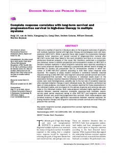
TABLE I A N O BSERVATION TABLE FOR A C ONSERVATIVE O PPONENT Strategy* CF CB BFC4 *

Ten 7.82 0 0 2.15 5

Observation Frequency Jack Queen King 8.75 9.08 1.34 0 0 0 0.25 0.29 0.29 5.83 14.3 18.55 3 2 1

Ace 0.01 0 17.17 0.17 0

B for bet; C for check; F for fold; C4 for all four players check and for represents no strategy taken.

face down. The first player can bet (adding one more chip) or check (doing nothing). When facing a bet, a player can also bet (adding one more chip) or fold to quit the current hand. A hand may end in a showdown either when everyone does not bet, or when all players respond to the first bet. In the latter case, only those who bet will join the showdown. During the showdown, the player with the largest card wins all chips on the table. A hand can also end without a showdown when only one player bets and all the others fold. In this case, the player who bets wins all chips. A new hand will start with another player becoming the first player, rotating in a clockwise order. The challenge of making an optimal decision in the 4-player Kuhn Poker game is threefold. The first challenge is caused by the uncertainty of opponents’ cards. For example, during one hand, opponents’ cards are unknown to each other, and even when the hand ends, the folded cards may still remain unrevealed. The second challenge is the uncertainty about the opponents’ strategies taken in each hand. Considering different kinds of players, such as bluffing players and conservative players, it is hard to predict the decisions those players may make in each hand. Lastly, compared to the traditional 2player Kuhn Poker game [13], the 4-player Kuhn Poker game introduces more complexity since a players’ strategy may be affected by the position/order of the player in one hand. Therefore, in this 4-player Kuhn Poker game, it is harder to predict opponents’ strategies due to the position constraints. B. Approach In this work, we explore how to solve decision making problems which involve uncertainty using probabilistic model checking techniques. The common solutions for such decision making problems include linear programming, dynamic programming or machine learning techniques. Those methods either require dedicated algorithms for different problems or have a high learning curve which causes difficulty for novices. The purpose of our approach is to explore the capability of model checking techniques to search for optimal decisions, which potentially reduce the learning curve as well as efforts of constructing and searching decision trees in the traditional methods. To handle uncertainty, our approach explores how to incorporate machine learning algorithms to derive insights from imperfect information so as to predict probabilistic distributions required in the user-specified models. In this way, we are able to utilize historical information to help make more accurate decisions. This enables us to tackle the challenges in dynamic environments. In particular, there are three components in our case study, i.e., opponent modeling,

poker game rule modeling and the best response decision, which we introduce in the following sections. 1) Opponent Modeling: The opponent modeling phase is an application of the machine learning component of our method in the 4-player Kuhn Poker game case study. We design an observation table for each opponent to record the frequencies of strategies taken by the opponent according to the card he/she holds. We adopt the Bayesian Inference [10] to compute the probability distributions of three opponents’ strategies providing the cards they hold as well as the probability distributions of the cards held by the opponents based on their observed betting strategies. Observation Table. Table I demonstrates a snapshot of the observation table for a conservative opponent. It is represented as a 2-dimensional matrix. Each row corresponds to the strategy an opponent can take, and each column corresponds to the card an opponent holds in a hand. A strategy consists of actions taken by an opponent in one hand. We use two bits to encode the strategies as the maximum number of turns a player can play is two in every hand. The betting strategy “CF” means the opponent checks in the 1st turn and folds in the 2nd turn. The strategy “CB” means the opponent checks in his/her 1st turn and bets in the 2nd turn. The strategy “B-” means that the opponent bets in his/her 1st turn and he would not have a chance to enter the 2nd turn. The strategy “F-” means that the opponent folds in the 1st turn and thus ends his action in this hand. We use “-” to represent no action is taken in that turn. “C4” is a special case meaning that all four players choose to check in their 1st turns, and thus the current hand ends after the 4th player checks. All four players will have to show their cards and the player with the largest card wins the game. Note that we record a full strategy in the observation table in order to infer the behavior of the player which may lead to the final winning/loosing result. Each cell shown in Table I records the count calculated based on an opponent’s card held and strategy taken in a hand that are observed/partially observed. Opponent Learning. Opponent learning in the 4-player Kuhn Poker game is real-time, and the observation table provides valuable insights into the opponent’s recent strategies. The opponent’s behavior is partially observed when our agent or he/she does not join a showdown as the card is not revealed. Definition 1 (Hand): A 4-player Kuhn Poker hand is a tuple H = (C, Cb , S, I, ObC) where C is the set of all five cards; Cb is the set of observed cards; S={CF, CB, B-, F-, C4} is the set of strategies; I is the set of opponents; ObC : I × C → {0, 1} represents whether a particular card held by an opponent is observed. 1 represents observed and 0 represents unobserved. At the end of a hand, the observation table will be updated according to the strategies and cards observed. Function F : I×C×S → R denotes the value to be added when updating the observation table. Obviously, this value depends on both the strategy taken by the opponent and the card he/she might have in this hand. The concrete update function F for opponent i who has card c using the strategy s is defined as follows.

( F(i, c, s) =

1

ObC(i, c) = 1

(1)

P(c | (i, s)) P 0 c0 ∈Cub P(c | (i, s))

ObC(i, c) = 0

(2)

where Cub = C − Cb is the set of unobserved cards. There are two scenarios that we may encounter at the end of a hand, i.e., an opponent’s card is observed and an opponent’s card is unobserved. In the first scenario, we increase the value of the cell in the observation table of opponent i, corresponding to card c by 1, as indicated in formula (1) in the definition of F. In the second scenario, we need to predict the possible card he/she is holding based on his/her current strategy taken and his/her observed historical information recorded in the observation table. In this case, the frequency F(i, c, s) is the ratio between the probability P(c | (i, s)) of holding a card c under the specified strategy s and the accumulated probabilities of holding all unobserved cards. Probability P(c | (i, s)) is calculated according to Bayesian inference shown below. P(c | (i, s)) =

P(s | (i, c))P(i, c) P(i, s)

P(i, s) is the probability of opponent i performing strategy s. The value of P(i, s) is 1 in this scenario since the strategy s of the opponent is observed. P(i, c) is the probability of opponent 1 i holding a card c. The value of P(i, c) is , meaning that | Cub |

the probability of opponent i holding any unobserved card c ∈ Cub is evenly distributed. P(s | (i, c)) is the probability of opponent i performing strategy s given that he/she holds card c. This probability is based on the historical observations recorded in the observation table, and its value is calculated Weight(i, c, s) by P , where Weight(i, c, s) denotes the fre0 s0 ∈S

Weight(i, c, s )

quency count of opponent i holding a card c under strategy s (cell (s, c) of component i’s observation table). Distribution. After learning from the opponents’ behavior history, our agent can predict the probability distribution of an opponent’s holding card based on his/her current strategy taken. Through the updated observation table, we can get the probability of opponent i holding a card c under strategy s through the following formula, Weight(i, c, s) 0 c0 ∈C Weight(i, c , s)

Pr(c | (i, s)) = P

All these probabilities constitute the opponent’s probabilistic distributions over holding a card (card probability distribution) and it is one input to the model checking component. Similarly, our agent can predict the probability distribution of the strategy which will be taken by an opponent based on his/her current card held. The probability of a strategy s that the opponent i holding a card c might take is calculated by the following formula, Pr(s | (i, c)) = P

Weight(i, c, s) Weight(i, c, s0 )

s0 ∈S

All the probabilities constitute the opponent’s bet probability distribution which is also input to the model checking stage.

2) Game Rule Modeling: The game rule modeling illustrates how to apply our probabilistic model checking component in the 4-player Kuhn Poker game. As a hand in this poker game progresses, each player will make a decision in turn. When it is our agent’s turn, it takes the response (i.e., bet or not) which maximizes the expected value through simulating all opponents’ possible strategies and cards. To achieve such a goal, we construct a probabilistic model to specify the poker game rules, followed by properties to be verified to derive probabilities of the chips that our agent may gain. We use the PCSP# modeling language to specify a hand of 4-player Kuhn Poker game. The PCSP# model covers three main parts: analyzing the card possibility of an opponent (process Simulate card(player) in Fig. 1), analyzing the action possibility based on an opponent’s possible card (process Betting phase(player)), and evaluating the winning chips of our agent in the current hand (process Evaluate). We remark that the probability distributions as the outcome of the machine learning stage will be used in processes Simulate card(player) and Betting phase(player). We illustrate one PCSP# process Simulate card(player) as an example, and the complete model is available at www.comp.nus.edu.sg/∼shiling/poker. Model for Card Possibility Analysis. In the process Simulate card(player) (shown in Fig. 1), the precondition requests that the current hand does not end and the opponent does not have a card (modeled by two if conditions in the first two lines). The PCSP# probabilistic choice operator pcase is used to capture all possible cards that an opponent may have. In our analysis, the probability of an opponent holding a card (e.g., ACE) is card prob[pos[player]][ACE] ∗ cards[ACE]/(card prob[pos[player]][ACE] ∗ cards[ACE] + · · · + card prob[pos[player]][TEN] ∗ cards[TEN]). The variable

card prob is declared as a 2-dimension array, and it records the probability of each card c for opponent i under the observed action(s), according to his/her past card probability distribution. The initialized probability of card prob is calculated based on the probability distribution from the machine learning stage in Section II-B1. The variable pos is an array which tracks the opponents’ index in the arrays card prob, and the variable cards is an array which records whether this card has been already occupied, value 0 for occupied, otherwise 1. The process Own(player, ACE) assigns the card ACE to the player. If this player has a card, then the process moves to the betting process Betting phase(player). When the current hand ends, the process moves to the evaluation process Evaluate. Verification Properties. We define six assertions to calculate the probabilities of our agent losing 1 or 2 chips, or winning 3, 4, 5, or 6 chips. These are all the possible situations that may happen at the end of a hand. One assertion is shown below. #define goalloss2 (player wins== − 2)&&(check==0); #assert kuhn poker reaches goalloss2 with prob;

The assertion derives the probability of the situation that the model for the Kuhn Poker game can reach a state where the

Simulate card(player) = if (!(player==first better&&game start)) { if (pos[player]! =(NUM PLAYERS − 1)&&player turns[player]==0){ pcase { card prob[pos[player]][ACE]∗cards[ACE] : Own(player, ACE) card prob[pos[player]][KING]∗cards[KING] : Own(player, KING) card prob[pos[player]][QUEEN]∗cards[QUEEN] : Own(player, QUEEN) card prob[pos[player]][JACK]∗cards[JACK] : Own(player, JACK) card prob[pos[player]][TEN]∗cards[TEN] : Own(player, TEN)} } else {Betting phase(player)} } else {Evaluate};

Fig. 1. Model for Card Possibility Analysis 280

No. of gained chips

240 200 160 120

80

𝑃1 𝐵 2 𝐵 3 𝐵 4 𝑃1 𝐵 2 𝐵 3 𝐶 4 𝑃1 𝐵 2 𝐶 3 𝐵 4 𝑃1 𝐵 2 𝐶 3 𝐶 4 𝑃1 𝐶 2 𝐵 3 𝐵 4 𝑃1 𝐶 2 𝐵 3 𝐶 4 𝑃1 𝐶 2 𝐶 3 𝐵 4 𝑃1 𝐶 2 𝐶 3 𝐶 4

40 0 -40 1 51 101151201251301351401451501551601651701751801851901951

No. of hands

Fig. 2. Performance of PATty over Conservative and Bluffing Players under 8 Configurations

condition goalloss2 is satisfied. Our agent calls the PAT model checker to exhaustively search the state space and calculate the probabilities of the states which satisfy the condition. 3) Best Response: The best response phase captures how to apply the decision making component of our method to the 4-player Kuhn Poker game case study. When it is our agent’s turn to make a decision during a hand, we compute the best response by calculating the maximum expected value (i.e., the highest gained chips) over all possible strategies we can adopt, based on the current and past hands’ observations. The expected value (EV) of the gained chips for strategy s is defined as P EV(s) = r∈R Prob(r | s) × r, where R = {−2, −1, 3, 4, 5, 6}, s = CB, B − or C4, where R is the set of all possible gained chips of our agent, and Prob(r | s) is the probability of winning r chips under strategy s corresponding to the assertion defined in Section II-B2. III. E XPERIMENTS In our experiment for the 4-player Kuhn Poker game, one agent (called P) simulates a player who adopts our method and the other three agents randomly mimic two types of players, namely, conservative player (called C) and bluffing player (called B). We run 10 games, and each game consists of 1000 hands. In each hand, each player plays based on the rules defined in Section II and all the players take turns to start the hands. After running the 10 games, the average performance across the 10 games is chosen for our analysis. Note that there is no limit for the number of chips that a player can bet in each game1 . 1 The detailed information of the experiments is available at www.comp. nus.edu.sg/∼shiling/poker.

The behaviors of the players are based on [11], where the behavior of the conservative player is similar to that of the tight-passive player, i.e., such a player participates in few hands, only considers playing those with a high probability of winning, and rarely raises the bet; the behavior of the bluffing player is similar to that of loose player, i.e., such a player often overestimates the hand and participates the bet. Our experiment considers all 8 configurations for 4 players in terms of their roles, i.e., P1 B2 B3 B4 , P1 B2 B3 C4 , P1 B2 C3 B4 , P1 B2 C3 C4 , P1 C2 B3 B4 , P1 C2 B3 C4 , P1 C2 C3 B4 , and P1 C2 C3 C4 , where superscripts 1, 2, 3 and 4 represent the player IDs. In all configurations, the first hand will start by Player 1; subsequently, the next hand will start by the player sitting next to the left-hand side of the player who starts in the previous hand. Figure 2 shows the gained chips of the player using our method (i.e., P) in all 8 configurations. The result indicates that P wins in all configurations by its learning capability and exhaustive search for an optimal decision. For example, in P1 C2 B3 C4 , P gradually wins the chips and ends up with a positive gain after it cumulatively learning opponents’ behaviors, despite its initial loss. IV. C ONCLUSION We conduct a case study with 4-player Kuhn Poker game by combining probabilistic model checking with machine learning. Experimental results show that the agent employing our method wins the most chips when playing against the conservative and bluffing players. R EFERENCES [1] W. L. Winston, Operations Research: Applications and Algorithms, 4th ed. Brooks/Cole, 2003. [2] J. S. Dong, L. Shi, L. V. N. Chuong, K. Jiang, and J. Sun, “Sports strategy analytics using probabilistic reasoning,” in ICECCS’2015, 2015, pp. 182–185. [3] S. J. Russell and P. Norvig, Artificial Intelligence - A Modern Approach (3rd Edition). Pearson Education, 2010. [4] A. Schrijver, Theory of Linear and Integer Programming. New York, NY, USA: John Wiley & Sons, Inc., 1986. [5] D. P. Bertsekas, Nonlinear Programming. Athena Scientific, 1999. [6] T. M. Mitchell, Machine Learning. McGraw-Hill, Inc., 1997. [7] E. M. Clarke, O. Grumberg, and D. A. Peled, Model Checking. The MIT Press, 1999. [8] P. Ballarini, M. Fisher, and M. Wooldridge, “Uncertain Agent Verification through Probabilistic Model-Checking,” in Safety and Security in Multiagent Systems. Springer, 2009, pp. 162–174. [9] A. Naskos, E. Stachtiari, P. Katsaros, and A. Gounaris, “Probabilistic model checking at runtime for the provisioning of cloud resources,” in Proceedings of the 15th International Conference on Runtime Verification (RV’2015), 2015, pp. 275–280. [10] G. E. P. Box and G. C. Tiao, Bayesian Inference in Statistical Analysis. Wiley-Interscience, 1973. [11] L. Barone and L. While, “Adaptive learning for poker,” in Proceedings of the 2Nd Annual Conference on Genetic and Evolutionary Computation, ser. GECCO’00, 2000, pp. 566–573. [12] M. Kwiatkowska, G. Norman, and D. Parker, “PRISM 4.0: Verification of probabilistic real-time systems,” in CAV’11, 2011, pp. 585–591. [13] H. W. Kuhn, “A Simplified Two-Person Poker,” in Contributions to the Theory of Games (AM-24), Volume I. Princeton University Press, 1950, pp. 97–104. [14] D. Szafron, R. Gibson, and N. Sturtevant, “A Parameterized Family of Equilibrium Profiles for Three-player Kuhn Poker,” in AAMAS ’13, 2013, pp. 247–254.