Feb 6, 2006 - Myla Archer and Shinya Umeno have helped me with PVS, proofs and strategies. Discussions with Dilsun Kaynar and Alexander Shvartsman ...
Translating Timed I/O Automata Specifications for Theorem Proving in PVS by
Hongping Lim Submitted to the Department of Electrical Engineering and Computer Science in partial fulfillment of the requirements for the degree of Master of Engineering in Electrical Engineering and Computer Science at the MASSACHUSETTS INSTITUTE OF TECHNOLOGY February 2006 c Massachusetts Institute of Technology 2006. All rights reserved.
Author . . . . . . . . . . . . . . . . . . . . . . . . . . . . . . . . . . . . . . . . . . . . . . . . . . . . . . . . . . . . . . . . . . . . . . . . . . . . Department of Electrical Engineering and Computer Science February 6, 2006
Certified by . . . . . . . . . . . . . . . . . . . . . . . . . . . . . . . . . . . . . . . . . . . . . . . . . . . . . . . . . . . . . . . . . . . . . . . . Nancy A. Lynch NEC Professor of Software Science and Engineering Thesis Supervisor
Accepted by . . . . . . . . . . . . . . . . . . . . . . . . . . . . . . . . . . . . . . . . . . . . . . . . . . . . . . . . . . . . . . . . . . . . . . . Arthur C. Smith Chairman, Department Committee on Graduate Students
Translating Timed I/O Automata Specifications for Theorem Proving in PVS by Hongping Lim Submitted to the Department of Electrical Engineering and Computer Science on February 6, 2006, in partial fulfillment of the requirements for the degree of Master of Engineering in Electrical Engineering and Computer Science
Abstract The timed input/output automaton modeling framework is a mathematical framework for specification and analysis of systems that involve discrete and continuous evolution. In order to employ an interactive theorem prover in deducing properties of a timed input/output automaton, its statetransition based description has to be translated to the language of the theorem prover. This thesis describes a tool for translating from TIOA, the formal language for describing timed input/output automata, to the language of the Prototype Verification System (PVS)—a specification system with an integrated interactive theorem prover. We describe the translation scheme, discuss the design decisions, and briefly present case studies to illustrate the application of the translator in the verification process. Thesis Supervisor: Nancy A. Lynch Title: NEC Professor of Software Science and Engineering
2
Acknowledgments I am grateful to Prof. Nancy Lynch for the opportunity to work with her, and for the excellent guidance and valuable help she has provided me with. I would like to thank the following members of the TIOA project. I am particularly grateful to Sayan Mitra with whom I worked closely throughout the development of the translator. His ideas and suggestions were integral to the design of the translator. Stephen Garland and Panayiotis Mavrommatis have provided me with much help on interfacing with the front-end type checker and intermediate-language parser. Myla Archer and Shinya Umeno have helped me with PVS, proofs and strategies. Discussions with Dilsun Kaynar and Alexander Shvartsman generated useful ideas for improving the translator.
3
Contents 1 Introduction 1.1 Motivation
9 . . . . . . . . . . . . . . . . . . . . . . . . . . . . . . . . . . . . . . . . .
9
1.2 Prior Work . . . . . . . . . . . . . . . . . . . . . . . . . . . . . . . . . . . . . . . . .
10
1.3 Thesis Overview . . . . . . . . . . . . . . . . . . . . . . . . . . . . . . . . . . . . . .
11
2 TIOA Mathematical Model and Language 2.1 TIOA Mathematical Model . . . . . . . . . . . . . . . . . . . . . . . . . . . . . . . .
13 13
2.1.1
Basic Definitions . . . . . . . . . . . . . . . . . . . . . . . . . . . . . . . . . .
13
2.1.2
Definition of Timed I/O Automata . . . . . . . . . . . . . . . . . . . . . . . .
14
2.1.3
Executions and Traces . . . . . . . . . . . . . . . . . . . . . . . . . . . . . . .
14
2.1.4
Composition . . . . . . . . . . . . . . . . . . . . . . . . . . . . . . . . . . . .
15
2.2 TIOA Language . . . . . . . . . . . . . . . . . . . . . . . . . . . . . . . . . . . . . .
16
3 Translation Scheme for Individual Automata
21
3.1 Data Types . . . . . . . . . . . . . . . . . . . . . . . . . . . . . . . . . . . . . . . . .
21
3.2 Automaton Parameters . . . . . . . . . . . . . . . . . . . . . . . . . . . . . . . . . .
25
3.3 Automaton States . . . . . . . . . . . . . . . . . . . . . . . . . . . . . . . . . . . . .
25
3.4 Actions and Transitions . . . . . . . . . . . . . . . . . . . . . . . . . . . . . . . . . .
25
3.4.1
Substitution Method . . . . . . . . . . . . . . . . . . . . . . . . . . . . . . . .
26
3.4.2
LET Method . . . . . . . . . . . . . . . . . . . . . . . . . . . . . . . . . . . .
29
3.4.3
Comparing the Substitution and LET Methods . . . . . . . . . . . . . . . . .
30
3.5 Trajectories . . . . . . . . . . . . . . . . . . . . . . . . . . . . . . . . . . . . . . . . .
31
3.6 Correctness of Translation . . . . . . . . . . . . . . . . . . . . . . . . . . . . . . . . .
33
3.7 Implementation . . . . . . . . . . . . . . . . . . . . . . . . . . . . . . . . . . . . . . .
34
4 Proving Properties in PVS
35
4.1 Case Studies . . . . . . . . . . . . . . . . . . . . . . . . . . . . . . . . . . . . . . . .
36
4.2 Invariant Proofs for Translated Specifications . . . . . . . . . . . . . . . . . . . . . .
39
4
4.3 Simulation Proofs for Translated Specifications . . . . . . . . . . . . . . . . . . . . . 5 Translating Specifications and Proving Properties of Composite Automata
41 46
5.1 Composite and Component Automata in TIOA . . . . . . . . . . . . . . . . . . . . .
47
5.2 Automaton Parameters and Component Formal Parameters . . . . . . . . . . . . . .
47
5.3 Automaton States . . . . . . . . . . . . . . . . . . . . . . . . . . . . . . . . . . . . .
49
5.3.1
Start States . . . . . . . . . . . . . . . . . . . . . . . . . . . . . . . . . . . . .
49
5.4 Actions and Transitions . . . . . . . . . . . . . . . . . . . . . . . . . . . . . . . . . .
50
5.4.1
Definitions for Input and Output Actions . . . . . . . . . . . . . . . . . . . .
50
5.4.2
Identifying Actions of the Composition . . . . . . . . . . . . . . . . . . . . . .
58
5.4.3
Predicates for Preconditions and Transitions . . . . . . . . . . . . . . . . . .
58
5.5 Trajectories . . . . . . . . . . . . . . . . . . . . . . . . . . . . . . . . . . . . . . . . .
59
5.6 Proving an Invariant of the LCR Leader Election Algorithm . . . . . . . . . . . . . .
62
6 Discussion and Future Work
65
6.1 Handling a Larger Class of Differential Equations . . . . . . . . . . . . . . . . . . . .
65
6.2 Improving Proofs and Developing Proof Strategies . . . . . . . . . . . . . . . . . . .
66
6.3 Developing a Library of User Defined Data Structures . . . . . . . . . . . . . . . . .
66
6.4 Developing a Repository of Complete Examples . . . . . . . . . . . . . . . . . . . . .
66
5
List of Figures 1-1 Theorem proving on TIOA specifications . . . . . . . . . . . . . . . . . . . . . . . . .
10
2-1 TIOA description of TwoTaskRace . . . . . . . . . . . . . . . . . . . . . . . . . . . .
18
2-2 Component automata for the LCR algorithm . . . . . . . . . . . . . . . . . . . . . .
19
2-3 Composite automaton for the LCR algorithm . . . . . . . . . . . . . . . . . . . . . .
20
3-1 PVS description of TwoTaskRace: states and actions declaration . . . . . . . . . . .
22
3-2 PVS description of TwoTaskRace: definitions for actions and trajectories . . . . . . .
23
3-3 PVS description of TwoTaskRace: definition for transition function . . . . . . . . . .
24
3-4 Actions and transitions in TIOA . . . . . . . . . . . . . . . . . . . . . . . . . . . . .
27
3-5 Translation of transitions using substitution . . . . . . . . . . . . . . . . . . . . . . .
27
3-6 Translation of transitions using let . . . . . . . . . . . . . . . . . . . . . . . . . . .
27
3-7 for loop in TIOA . . . . . . . . . . . . . . . . . . . . . . . . . . . . . . . . . . . . . .
28
3-8 Translation of for loop using substitution . . . . . . . . . . . . . . . . . . . . . . . .
28
3-9 Translation of for loop using let . . . . . . . . . . . . . . . . . . . . . . . . . . . . .
28
3-10 Differential inclusion in TIOA . . . . . . . . . . . . . . . . . . . . . . . . . . . . . . .
32
3-11 Using an additional parameter to specify rate of evolution . . . . . . . . . . . . . . .
32
4-1 TIOA and PVS descriptions of the mutual exclusion property . . . . . . . . . . . . .
37
4-2 TIOA description of TwoTaskRaceSpec . . . . . . . . . . . . . . . . . . . . . . . . . .
37
4-3 TIOA description of simulation relation from TwoTaskRace to TwoTaskRaceSpec . .
38
4-4 Proof tree for proving an invariant of TwoTaskRace . . . . . . . . . . . . . . . . . . .
40
4-5 An invariant of TwoTaskRace . . . . . . . . . . . . . . . . . . . . . . . . . . . . . . .
40
4-6 PVS description of TwoTaskRaceSpec . . . . . . . . . . . . . . . . . . . . . . . . . .
43
4-7 PVS description of TwoTaskRaceSpec (continued) . . . . . . . . . . . . . . . . . . . .
44
4-8 PVS description of the simulation relation from TwoTaskRace to TwoTaskRaceSpec .
45
5-1 PVS translation for LCR: automaton parameters and states . . . . . . . . . . . . . .
48
5-2 PVS translation for LCR: definitions for transitions of Process . . . . . . . . . . . .
51
6
5-3 PVS translation for LCR: definitions for transitions of Channel . . . . . . . . . . . .
52
5-4 PVS translation for LCR: actions declaration . . . . . . . . . . . . . . . . . . . . . .
53
5-5 PVS translation for LCR: time passage predicate and where clause . . . . . . . . . .
54
5-6 PVS translation for LCR: transition predicates . . . . . . . . . . . . . . . . . . . . .
55
5-7 PVS translation for LCR: enabled clauses . . . . . . . . . . . . . . . . . . . . . . . .
56
5-8 PVS translation for LCR: enabled predicate and transition function . . . . . . . . . .
57
5-9 Trajectories in TIOA . . . . . . . . . . . . . . . . . . . . . . . . . . . . . . . . . . . .
60
5-10 Translation of trajectories for composition . . . . . . . . . . . . . . . . . . . . . . . .
61
5-11 An invariant of the LCR algorithm . . . . . . . . . . . . . . . . . . . . . . . . . . . .
63
7
List of Tables 3.1 Translation of program statements. . . . . . . . . . . . . . . . . . . . . . . . . . . . .
8
26
Chapter 1
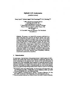
Introduction The timed input/output automaton [10, 9] modeling framework is a mathematical framework for compositional modeling and analysis of systems that involve discrete and continuous evolution. The state of a timed I/O automaton changes discretely through actions, and continuously over time intervals through trajectories. A formal language called TIOA [8, 7] has been designed for specifying timed I/O automata. The TIOA language subsumes its predecessor, the IOA language [6], which was developed earlier for specification of purely discrete distributed systems. In the TIOA language, discrete transitions are specified in a precondition-effect style. In addition, TIOA introduces new constructs for specifying trajectories. Based on the TIOA language, a set of software tools is being developed [8]; these tools include (1) a front-end type checker, (2) a simulator, and (3) an interface to the Prototype Verification System (PVS) theorem prover [19] (see Figure 1-1). This thesis describes the new features of the TIOA language and a tool for translating specifications written in TIOA to the language of PVS; this tool is a part of the third component of the TIOA toolkit.
1.1
Motivation
Verification of timed I/O automata properties typically involves proving invariants of individual automata or proving simulation relations between pairs of automata. The key technique for proving both invariants and simulation relations for state-machine models like the timed I/O automata is induction. The timed I/O automata framework provides a means for constructing very stylized proofs, which take the form of induction over the length of the executions of an automaton or a pair of automata, and a systematic case analysis of the actions and the trajectories. Therefore, it is possible to partially automate such proofs by using an interactive theorem prover, as shown in [1]. Apart from partial automation, theorem prover support is also useful for managing large proofs, and for re-checking proofs after minor changes in the specification. We have chosen to use the PVS theorem prover because it provides an expressive specification 9
TIOA file automaton A invariants of A automaton B invariants of B forward simulation from A to B
TIOA Toolkit Frontend
Intermediate Language
Translator
Other tools (E.g. Simulator)
A_decls.pvs A_invariants.pvs
PVS
B_decls.pvs B_invariants.pvs A2B.pvs
TIOA Library time.pvs time_thy.pvs time_machine.pvs
timed_automaton.pvs forward_simulation.pvs pvs−strategies auto_induct deadline_check try_simp
Figure 1-1: Theorem proving on TIOA specifications language and an interactive theorem prover with powerful decision procedures. PVS also provides a way of developing special strategies or tactics for partially automating proofs, and it has been used in many real life verification projects [20]. To use a theorem prover like PVS for verification, one has to write the description of the timed I/O automaton model of the system in the language of PVS, which is based on classical, typed higher-order logic. One could write this automaton specification directly in PVS, but using the TIOA language has the following advantages: 1. TIOA preserves the state-transition structure of a timed I/O automaton, 2. TIOA allows the user to write programs to describe the transitions using operational semantics, whereas in PVS, transition definitions have to be functions or relations, 3. TIOA provides a natural way for describing trajectories using differential equations, and also, 4. TIOA allows one to use other tools in the TIOA toolkit. Therefore, it is desirable to be able to write the description of a timed I/O automaton in the TIOA language, and then use an automated tool to translate this description to the language of PVS.
1.2
Prior Work
Various tools have been developed to translate IOA specifications to different theorem provers, for example, Larch [3, 5], PVS [4], and Isabelle [18, 21]. Our implementation of the TIOA to PVS translator builds upon [3]. The IOA language is designed for specification of I/O automata that evolve only through discrete actions. However, unlike IOA, TIOA allows the state of a timed I/O automaton to evolve continuously over time through trajectories. The Timed Automata Modeling Environment (TAME) [1] provides a PVS theory template for describing MMT automata [14]— an extension of I/O automaton that adds time bounds for enabled 10
actions. This theory template has to be manually instantiated with the states, actions, and transitions of an automaton. A similar template is instantiated automatically by our translator to specify timed I/O automata in PVS. This entails translating the operational descriptions of transitions in TIOA to their corresponding functional descriptions in PVS. Moreover, unlike a timed I/O automaton which uses trajectories, an MMT automaton uses time passage actions to model continuous behavior. In TAME, a time passage action is written as another action of the automaton, with the properties of the pre-state and post-state expressed in the enabling condition of the action. This approach, however, if applied directly to translate a trajectory, does not allow assertion of properties that must hold throughout the duration of the trajectory. Our translation scheme solves this problem by embedding the trajectory as a functional parameter of the time passage action.
1.3
Thesis Overview
The main contribution of this thesis is the design of a translation scheme from TIOA to PVS, and the implementation of the translator. We illustrate the application of the translator in the following four case studies: Fischer’s mutual exclusion algorithm, a two-task race system, a simple failure detector, and the LCR leader election algorithm [11, 9]. The TIOA specifications of the system and its properties are given as input to the translator and the output from the translator is a set of PVS theories, specifying the timed I/O automaton and its invariant properties. The PVS theorem prover is then used to verify the properties using inductive invariant proofs. In two of these case studies, we describe time bounds on the actions of interest using an abstract automaton, and then show the timing properties by proving a simulation relation from the system to this abstraction [12]. The simulation relations typically involve inequalities between variables of the system and its abstraction. Our experience with the tool suggests that the process of writing system descriptions in TIOA and then proving system properties using PVS on the translator output can be helpful in verifying more complicated systems. We also present an approach to handling composition using the translator, in which sets of automata are composed into a larger system [11, 9, 22]. The input to the translator consists of descriptions of the individual automata and a composite automaton which describes how the component automata are composed together. The output of the translator is a single system in PVS representing the composition of the components. Our approach is similar to that of the composer of the IOA compiler [22]. The composer of the IOA compiler expands a composite automaton definition into an equivalent individual automaton within IOA so that it can be used with other tools in the IOA toolkit. For our translation, we are able to make use of the language features of PVS to produce a more structured and layered expansion of a composite automaton in PVS for the purpose of theorem-proving. In particular, PVS allows us to write definitions to specify predicates
11
and functions – this feature is not available in IOA. The use of definitions and naming conventions avoids potential naming conflicts and helps present the composition operation in a clear modular manner. To illustrate the translation scheme for composition, we have successfully translated the LCR leader election algorithm using the TIOA to PVS translator, and verified an invariant of the algorithm using PVS. In the next chapter, we give a brief overview of the timed I/O automaton framework and the TIOA language. In Chapter 3, we present the translation scheme for translating TIOA descriptions into PVS specifications and describe the implementation of the translator. In Chapter 4, we illustrate the application of the translator with brief overviews of the case studies that do not involve composition. We present the translation scheme for composition in Chapter 5. Finally, Chapter 6 provides a brief discussion and suggests possible areas of improvements to the translation and theorem proving process. The translator tool, together with the files for the case studies and additional documentation can be obtained at the following address: http://theory.csail.mit.edu/~hongping/tioa2pvs.
12
Chapter 2
TIOA Mathematical Model and Language In this chapter, we briefly describe the timed I/O automaton model and the TIOA language. We refer the reader to [10] for a complete description of the mathematical framework, and to [8] for the TIOA user guide and reference manual.
2.1 2.1.1
TIOA Mathematical Model Basic Definitions
If f is a function, then we denote the domain of f by dom(f ). If S is a set, then f d S denotes the restriction of f to S, that is, the function g with dom(g) = dom(f ) ∩ S such that g(c) = f (c) for each c ∈ dom(g). Let V be the set of variables of a system. Each variable v ∈ V is associated with a static type, type(v), which is the set of values v can assume. A valuation for V is a function that associates each variable v ∈ V to a value in type(v). val(V ) denotes the set of all valuations of V . Each variable v ∈ V is also associated with a dynamic type, which is the set of trajectories v may follow. A time interval J is a nonempty, left-closed sub-interval of R. J is said to be closed if it is also right-closed. A trajectory τ of V is a mapping τ : J → val(V ), where J is a time interval starting with 0. The domain of τ , τ.dom, is the interval J. A point trajectory is one with the trivial domain {0}. The first time of τ , τ.f time, is the infimum of τ.dom. If τ.dom is closed then τ is closed and its limit time, τ.ltime, is the supremum of τ.dom. For any variable v ∈ V , τ ↓ v(t) denotes the restriction of τ to the set val(v). τ.f val is the first valuation of τ . If τ is closed, τ.lval is the last valuation. τ.f state denotes the first state of τ , and if τ is closed, τ.lstate denotes the last state. Let τ and τ 0 be trajectories for V , with τ closed. The concatenation of τ and τ 0 is the union of τ and 13
the function obtained by shifting τ 0 .dom until τ.ltime = τ 0 .f time. The suffix of a trajectory τ is obtained by restricting τ.dom to [t, ∞), and then shifting the resulting domain by −t.
2.1.2
Definition of Timed I/O Automata
A timed automaton B is a tuple of (X, Q, Θ, E, H, D, T ) where: 1. X is a set of variables. 2. Q ⊆ val(X) is a set of states. 3. Θ ⊆ Q is a nonempty set of start states. 4. A is a set of actions, partitioned into external E and internal actions H. 5. D ⊆ Q × A × Q is a set of discrete transitions. We write a transition (x, a, x 0 ) ∈ D in short as a
a
x → x0 . We say that a is enabled in x if x → x0 for some x0 . 6. T is a set of trajectories for X such that τ (t) ∈ Q for every τ ∈ T and every t ∈ τ.dom, and T is closed under prefix, suffix and concatenation. A timed I/O automaton is a timed automaton with the set of external actions E further partitioned into input and output actions. A timed I/O automaton A is a tuple (B, I, O) where: 1. B = (X, Q, Θ, E, H, D, T ) is a timed automaton. 2. I and O partition E into input and output actions, respectively. 3. The following additional axioms are satisfied: (a) (Input action enabling) a
For every x ∈ Q and every a ∈ I, there exists x0 ∈ Q such that x → x0 . (b) (Time-passage enabling) For every x ∈ Q, there exists τ ∈ T such that τ.f state = x and either i. τ.ltime = ∞, or ii. τ is closed and some l ∈ H ∪ O is enabled in τ.lstate.
2.1.3
Executions and Traces
An execution fragment of a timed I/O automaton A is an alternating sequence of actions and trajectories α = τ0 a1 τ1 a2 . . ., where τi ∈ T , ai ∈ A, and if τi is not the last trajectory in α then τi is ai+1
finite and τi .lstate → τi+1 .f state. Informally, an execution fragment records what happens during a particular run of a system. It includes all the discrete state changes and all the changes that occur 14
while time advances. An execution fragment is closed if it is a finite sequence and the domain of the final trajectory is a finite closed interval. An execution is an execution fragment whose first state is a start state of A. A state of A is reachable if it is the last state of some execution. An invariant property is one which is true in all reachable states of A. A trace of an execution fragment α is obtained from α by removing internal actions and modifying the trajectories to contain only information about the amount of elapsed time. traces A denotes the set of all traces of A. We say that timed I/O automaton A implements timed I/O automaton B if traces A ⊆ tracesB . A forward simulation relation [10] from A to B is a sufficient condition for showing that A implements B. A forward simulation from automaton A to B is a relation R ⊆ QA × QB satisfying the following conditions for all states xA ∈ QA and xB ∈ QB : 1. If xA ∈ ΘA then there exists a state xB ∈ ΘB such that xA R xB . a
2. If xA R xB and α is a transition x →A x0 , then B has a closed execution fragment β with β.f state = xB , trace(β) = trace(α), and α.lstate R β.lstate. 3. If xA R xB and α is an execution fragment of A consisting of a single closed trajectory, with α.f state = xA , then B has a closed execution fragment β with β.f state = xB , trace(β) = trace(α), and α.lstate R β.lstate.
2.1.4
Composition
We first describe the composition operation for timed automata, and then for timed I/O automata. Composition allows an automaton representing a complex system to be constructed by composing together individual components. The composition operation identifies external actions with the same name in different component automata in the following way. When any component automaton performs a discrete action a, all component automata that have a as an external action will also perform a simultaneously. Formally, timed automata B1 and B2 are compatible if H1 ∩ A2 = H2 ∩ A1 = ∅ and X1 ∩ X2 = ∅. If B1 and B2 are compatible, then their composition, denoted by B1 k B2 , is defined to be the tuple B = (X, Q, Θ, E, H, D, T ) where: 1. X = X1 ∪ X2 . 2. Q = {x ∈ val(X) | x d Xi ∈ Qi , i ∈ {1, 2}}. 3. Θ = {x ∈ Q|x ∈ Θi , i ∈ {1, 2}}. 4. E = E1 ∪ E2 and H = H1 ∪ H2 . 15
a
5. For each x, x0 ∈ Q and each a ∈ A, x →A x0 iff for i ∈ {1, 2}, either a
(a) a ∈ Ai and x d Xi →i x0 , or (b) a ∈ / Ai and x d Xi = x0 d Xi . 6. T ⊆ trajs(X) is given by τ ∈ T ⇔ τ ↓ Xi ∈ Ti , i ∈ {1, 2}. As shown in [10], the result of composing two timed automata is guaranteed to be a timed automaton. Composition for timed I/O automata is based on the above definition for timed automata, taking into consideration the input and output distinction. Timed I/O automata A1 and A2 are compatible if, for i 6= j, Xi ∩ Xj = Hi ∩ Aj = Oi ∩ Oj = ∅ 1 . If A1 = (B1 , I1 , O1 ) and A2 = (B2 , I2 , O2 ) are compatible, then their composition, denoted by A1 k A2 , is defined to be the tuple A = (B, I, O) where 1. B = B1 k B2 2. I = (I1 ∪ I2 ) − (O1 ∪ O2 ) 3. O = O1 ∪ O2 An external action a of the composition is classified as an output action if a is an output of one of the component automata. Otherwise, a is an input action. As shown in [10], the composition of two timed I/O automata is guaranteed to be a timed I/O automaton.
2.2
TIOA Language
The TIOA language [8] is a formal language for specifying the components and properties of timed I/O automata. The states, actions and transitions of a timed I/O automaton are specified in TIOA in the same way as in the IOA language [6]. New features of the TIOA language include trajectories, a new AugmentedReal data type, and a new vocabulary syntax for specifying user-defined data types and operators. The trajectories are defined using differential and algebraic equations, invariants and stopping conditions. This approach is derived from [13], in which the authors had used differential equations and English to describe trajectories informally . The AugmentedReal type extends reals with a constructor for infinity. Each variable has an explicitly defined static type, and an implicitly defined dynamic type. The dynamic type of a Real variable is the set of piecewise-continuous functions; the dynamic type of a variable of any other simple type or of the type discrete Real is the set of piecewise constant functions. 1 Relaxing the constraints by removing the requirement O ∩ O = ∅ will still yield a timed I/O automaton as the i j result of the composition.
16
The set of trajectories of a timed I/O automaton is defined systematically by a set of trajectory definitions. A trajectory definition w is defined by an invariant inv(w), a stopping condition stop(w), and a set of differential and algebraic equations daes(w). Let WA denote the set of trajectory definitions of A. Each trajectory definition w ∈ WA defines a set of trajectories, denoted by traj(w). A trajectory τ belongs to traj(w) if the following conditions hold. For each t ∈ τ.dom: 1. τ (t) ∈ inv(w). 2. If τ (t) ∈ stop(w), then t = τ.ltime. 3. τ (t) satisfies the set of differential and algebraic equations in daes(w). 4. For each non-real variable v, (τ ↓ v)(t) = (τ ↓ v)(0); that is, the value of v is constant throughout the trajectory.
S
The set of trajectories TA of automaton A is the concatenation closure of the functions in w∈WA
traj(w).
Figures 2-1 and 2-2 show three examples of TIOA specifications. The automaton keyword declares the name of the automaton, together with any automaton parameters and a where clause constraining the values of the parameters. The signature keyword declares the actions, specifying whether each action is internal, or external (input or output). State variables are declared using the states keyword, together with their types and initial values. Transitions are specified by the transitions keyword. Each transition has a precondition (pre) and an effect ( eff ). The trajectories keyword specifies trajectory definitions (trajdef). Each trajectory definition has an invariant, a stopping condition specified by stop when, and an evolve clause stating the evolution of variables. Figure 2-3 shows an example of a composite automaton consisting of component automata of types Process and Channel from Figure 2-2. These examples will be referenced again and discussed further in subsequent chapters.
17
2 4 6 8 10 12 14 16 18 20 22 24 26 28 30 32 34 36 38 40 42 44
automaton TwoTaskRace(a1 , a2 , b1 , b2 : Real ) where a1 > 0 ∧ a2 > 0 ∧ b1 ≥ 0 ∧ b2 > 0 ∧ a2 ≥ a1 ∧ b2 ≥ b1 signature i n t e r n a l increment i n t e r n a l decrement i n t e r n a l set output report states count : Int := 0 , flag : Bool := false , reported: Bool := false , now : Real := 0 , first_main : Real := a1 , last_main : AugmentedReal := a2 , first_set : Real := b1 , last_set: AugmentedReal := b2 transitions i n t e r n a l increment pre ¬flag ∧ now ≥ first_main e f f count := count + 1; first_main := now + a1 ; last_main := now + a2 i n t e r n a l set pre ¬flag ∧ now ≥ first_set e f f flag := true ; first_set := 0; last_set := \ infty i n t e r n a l decrement pre flag ∧ count > 0 ∧ now ≥ first_main e f f count := count - 1; first_main := now + a1 ; last_main := now + a2 output report pre flag ∧ count = 0 ∧ ¬reported ∧ now ≥ first_main e f f reported := true ; first_main := 0; last_main := \ infty trajectories t r a j d e f traj1 i n v a r i a n t now ≥ 0 stop when now = last_main ∨ now = last_set evolve d( now ) = 1 Figure 2-1: TIOA description of TwoTaskRace
18
2 4 6 8 10 12 14 16 18 20 22 24 26 28 30 32 34 36 38
automaton Process( index , n: Int) imports RingVocab signature input receive(m : Int , h : Int , i : Int ) where h = mod (i - 1 , n ) ∧ i = index output send (m : Int , i: Int , j: Int) where j = mod (i + 1 , n ) ∧ i = index output leader (i: Int ) where i = index states pending: Seq [ Int ] := {} ` id ( index ) , status : Status := waiting transitions input receive(m: Int , h: Int , i: Int ) e f f i f ( m > id ( i )) then pending:= pending ` m e l s e i f ( m = id (i )) then status := elected fi output send (m : Int , i : Int , j : Int ) pre pending 6= {} ∧ m = head ( pending) e f f i f pending 6= {} then pending:= tail ( pending) f i output leader (z) pre status = elected e f f status := announced automaton Channel( sender , receiver: Int ) signature input send (m : Int , i : Int , j : Int ) where i = sender ∧ j = receiver output receive(m: Int , i : Int , j : Int ) where i = sender ∧ j = receiver states buffer : Seq [ Int ] := {} transitions output receive(m: Int , i : Int , j : Int ) pre buffer 6= {} ∧ m = head ( buffer ) e f f i f buffer 6= {} then buffer := tail ( buffer ) f i input send (m , i , j) e f f buffer := buffer ` m Figure 2-2: Component automata for the LCR algorithm
19
vocabulary RingVocab types Status enumeration [ waiting , elected , announced] operators mod : Int , Int → Int id : Int → Int automaton LCR( n : Int ) where n > 0 imports RingVocab components P[i: Int ]: Process(i , n) where 0 ≤ i ∧ i < n; C[x: Int ]: Channel(x , mod (x + 1 , n )) where 0 ≤ x ∧ x < n Figure 2-3: Composite automaton for the LCR algorithm
20
Chapter 3
Translation Scheme for Individual Automata In this chapter, we provide an overview of our approach for translation, and then give details of how we translate the various components of a TIOA description. For generating PVS theories that specify input TIOA descriptions, our translator implements the approach prescribed in TAME [1]. The translator instantiates a predefined PVS theory template that defines the components of a generic automaton. The translator automatically instantiates the template with the states, actions, and transitions of the input TIOA specification. This instantiated theory, together with several supporting library theories, completely specifies the automaton, its transitions, and its reachable states in the language of PVS (see Figure 1-1). Figures 3-1, 3-2, and 3-3 show the translator output in PVS for the TIOA description in Figure 2-1. Lines 123–125 of Figure 3-3 show how the translation output in PVS instantiates the time machine template with the definitions of the various components of the automaton. In the following sections, we describe the translation of the various components of a TIOA description.
3.1
Data Types
Simple static types of the TIOA language Bool, Char, Int, Nat, Real and String have their equivalents in PVS. PVS also supports declaration of TIOA types enumeration, tuple, union, and array in its own syntax. The type AugmentedReal is translated to the type time introduced in the time theory of TAME. The type time is defined as a datatype consisting of two subtypes: fintime and infinity. The subtype fintime consists of only non-negative reals, while infinity is a constant constructor. The TIOA language allows the user to introduce new types and operators by declaring the types
21
T w o T a s k R a c e d e c l s : THEORY BEGIN 2
IMPORTING common decls 4
% Automaton p a r a m e t e r s a1 : r e a l a2 : r e a l 8 b1 : r e a l b2 : r e a l 6
10 12
% Where c l a u s e on p a r a m e t e r s t r a n s l a t e d as axiom TwoTaskRace params ax : AXIOM a1 > 0 AND a2 > 0 AND b1 ≥ 0 AND b2 > 0 AND a2 ≥ a1 AND b2 ≥ b1
14 16 18 20 22 24 26 28 30 32 34
% State variables s t a t e s : TYPE = [# count : int , f l a g : bool , r e p o r t e d : bool , now : r e a l , first main : real , l a s t m a i n : time , f i r s t s e t : real , l a s t s e t : t i m e #] % Start state s t a r t ( s : s t a t e s ) : b o o l = s=s WITH [ count := 0 , f l a g := f a l s e , r e p o r t e d := f a l s e , now : = 0 , f i r s t m a i n : = a1 , l a s t m a i n : = f i n t i m e ( a2 ) , f i r s t s e t : = b1 , l a s t s e t : = f i n t i m e ( b2 ) ]
36
f t y p e ( i , j : ( f i n t i m e ? ) ) : TYPE = [ i n t e r v a l ( i , j )→s t a t e s ] 38 40 42 44 46 48
% Actions s i g n a t u r e s a c t i o n s : DATATYPE BEGIN n u t r a j 1 ( d e l t a t : { t : ( f i n t i m e ? ) | d u r ( t )≥0 } , F : f t y p e ( zero , d e l t a t ) ) : nu traj1 ? increment : increment? decrement : decrement ? set : set ? report : report ? END a c t i o n s Figure 3-1: PVS description of TwoTaskRace: states and actions declaration
22
% actions v i s i b i l i t y v i s i b l e ( a : a c t i o n s ) : b o o l = CASES a OF 51 n u t r a j 1 ( d e l t a t , F ) : FALSE, i n c r e m e n t : FALSE, 53 d e c r e m e n t : FALSE, s e t : FALSE, 55 r e p o r t : TRUE ENDCASES 49
57
% time p a s s a g e a c t i o n s t i m e p a s s a g e a c t i o n s ( a : a c t i o n s ) : b o o l = CASES a OF n u t r a j 1 ( d e l t a t , F ) : TRUE, 61 i n c r e m e n t : FALSE, d e c r e m e n t : FALSE, 63 s e t : FALSE, r e p o r t : FALSE 65 ENDCASES
59
67
% Clauses f o r t r a j e c t o r y d e f i n i t i o n t r a j 1 t r a j 1 i n v a r i a n t ( s : s t a t e s ) : b o o l = TRUE
69 71 73
tr aj 1 st op ( s : states ) : bool = f i n t i m e ( now ( s ) ) = l a s t m a i n ( s ) OR f i n t i m e ( now ( s ) ) = l a s t s e t ( s ) traj1 evolve ( t : ( fintime ?) , s : states ) : states = s WITH [ now : = now ( s ) + 1 ∗ d u r ( t ) ]
75 77 79 81 83 85 87 89 91
% Enabled enabled (a : actions , s : states ) : bool = CASES a OF nu traj1 ( delta t , F): (FORALL ( t : i n t e r v a l ( z e r o , d e l t a t ) ) : t r a j 1 i n v a r i a n t ( s ) ) AND (FORALL ( t : i n t e r v a l ( z e r o , d e l t a t ) ) : t r a j 1 s t o p (F( t ) ) ⇒ t = d e l t a t ) AND (FORALL ( t : i n t e r v a l ( z e r o , d e l t a t ) ) : F( t ) = t r a j 1 e v o lv e ( t , s )) i n c r e m e n t : NOT f l a g ( s ) AND now ( s ) ≥ f i r s t m a i n ( s ) , d e c r e m e n t : f l a g ( s ) AND c o u n t ( s ) > 0 AND now ( s ) ≥ f i r s t m a i n ( s ) , s e t : NOT f l a g ( s ) AND now ( s ) ≥ f i r s t s e t ( s ) , report : flag (s) AND c o u n t ( s ) = 0 AND NOT r e p o r t e d ( s ) AND now ( s ) ≥ f i r s t m a i n ( s )
93
ENDCASES Figure 3-2: PVS description of TwoTaskRace: definitions for actions and trajectories
23
95 97
% Transition function trans (a : actions , s : states ): states = CASES a OF nu traj1 ( delta t , F ) : F( d el t a t ) ,
99 101 103 105 107
increment : LET s=s WITH [ c o u n t : = c o u n t ( s ) + 1 ] IN LET s=s WITH [ f i r s t m a i n : = now ( s ) + a1 ] IN LET s=s WITH [ l a s t m a i n : = f i n t i m e ( now ( s ) + a2 ) ] IN s , decrement : LET s=s WITH [ c o u n t : = c o u n t ( s ) − 1 ] IN LET s=s WITH [ f i r s t m a i n : = now ( s ) + a1 ] IN LET s=s WITH [ l a s t m a i n : = f i n t i m e ( now ( s ) + a2 ) ] IN s ,
109 111 113 115 117
set : LET s=s WITH [ f l a g : = t r u e ] IN LET s=s WITH [ f i r s t s e t : = 0 ] IN LET s=s WITH [ l a s t s e t : = i n f i n i t y ] IN s , report : LET s=s WITH [ r e p o r t e d : = t r u e ] IN LET s=s WITH [ f i r s t m a i n : = 0 ] IN LET s=s WITH [ l a s t m a i n : = i n f i n i t y ] IN s
119
ENDCASES 121
% Import s t a t e m e n t s 123 IMPORTING t i m e d a u t o l i b @ t i m e m a c h i n e 125
[ states , actions , enabled , trans , s t a r t , v i s i b l e , timepassageactions , lambda ( a : { x : a c t i o n s | t i m e p a s s a g e a c t i o n s ( x ) } ) : d u r ( d e l t a t ( a ) ) ]
127 END T w o T a s k R a c e d e c l s
Figure 3-3: PVS description of TwoTaskRace: definition for transition function
24
and the signatures of the operators within the TIOA description using the keyword vocabulary. The semantics of these types and operators are written in PVS library theories, which are imported by the translator output.
3.2
Automaton Parameters
An automaton can be parameterized; the automaton parameters can be used in expressions within the description of the automaton. The values of these automaton parameters can be constrained with an optional where clause (see Figure 2-1, lines 1–4). In PVS, automaton parameters are declared as constants with axioms stating the relationship among them as specified by the where clause (see Figure 3-1, lines 5–13).
3.3
Automaton States
The TIOA language provides the construct states for declaring the state variables of an automaton (see Figure 2-1, lines 11–19). Each variable can be assigned an initial value at the start state. An optional initially predicate can be used to specify the possible values of the variables in a start state. In PVS, the state of an automaton is defined as a record with fields corresponding to the variables of the automaton (see Figure 3-1, lines 16–24). A boolean predicate start returns true when a given state satisfies the conditions of a start state (see Figure 3-1, lines 27–35). Assignments of initial values to variables in the TIOA description are translated as a record equality in the start predicate in PVS, while the initially predicate is inserted as an additional conjunction clause into the start predicate.
3.4
Actions and Transitions
In TIOA, actions are declared as internal or external (input or output). In PVS, actions are declared as subtypes of an actions datatype. A visible predicate returns true for the external actions. In TIOA, discrete transitions are specified in precondition-effect style using the keyword pre followed by a predicate (precondition), and the keyword eff followed by a program (effect) (see Figure 2-1, lines 20–40). We define a predicate enabled in PVS parameterized on an action a and a state s to represent the preconditions. The predicate enabled returns true when the corresponding TIOA precondition for an action a is satisfied at state s. The program of the effect clause specifies the relation between the post-state and the pre-state of the transition. The program consists of sequential statements, which may be assignments, if 25
program P
transP (s)
v := t
s with [v := t]
if pred then P1 fi
if pred then transP1 (s) else s endif
if pred then P1 else P2 fi
if pred then transP1 (s) else transP2 (s) endif
for v in A do P1 od
forloop(A, s): recursive states = if empty?(A) then s else let v=choose(A), s’=forloop(remove(v, A), s) in transP 1 (s’) endif measure card(A) Table 3.1: Translation of program statements.
then-else conditionals or for loops. A non-deterministic assignment is handled by adding extra parameters to the action declaration and constraining the values of these parameters in the enabled predicate of the action. In TIOA, the effect of a transition is typically written in an imperative style using a sequence of statements. We translate each type of statement to its corresponding functional relation between states, as shown in Table 3.1. The term P is a program, while transP (s) is a function that returns the state obtained by performing program P on state s. The term v is a state variable; t is an expression, and its value is assigned to v; pred is a predicate of the conditional statement; A is a finite set containing the set of elements the for loop iterates over. The PVS keyword with makes a copy of the record s, assigning the field v with a new value t. The PVS function choose picks an arbitrary element from the given set A. In PVS, we define a function trans parameterized on an action a and a state s, which returns the post-state of performing the corresponding TIOA effect of action a on state s. Sequential statements like P1 ; P2 are translated to a composition of the corresponding functions transP2 (transP1 (s)). Our translator can perform this composition in two ways. The first approach obtains an expression for the final value of each variable through a series of substitutions. The second approach composes the sequence of functions together using the PVS let keyword. When using the translator, the user can specify which translation method to use to translate all the transitions of an automaton.
3.4.1
Substitution Method
Given a sequential program consisting of two smaller programs P1 and P2 , we first compute transP1 . Then, we replace each variable in transP2 with its intermediate value obtained from transP1 . This approach explicitly specifies the resulting value of each variable in the post-state in terms of the variables in the pre-state [3].
26
automaton A signature i n t e r n a l foo (i : Int ) , bar states x , y , t: Int transitions i n t e r n a l foo (i : Int ) i n t e r n a l bar e f f x := x + i ; e f f t := x; y := x * x ; i f x 6= y then x := x - 1; x := y; y := y + 1 y := t fi Figure 3-4: Actions and transitions in TIOA
t r a n s ( a : a c t i o n s , s : s t a t e s ) = CASES a OF f o o ( i ) : s WITH [ x : = x ( s ) + i − 1 , y := ( x ( s ) + i ) ∗ ( x ( s ) + i ) + 1 ] , b a r : s WITH [ y : = IF x ( s ) /= y ( s ) THEN x(s) ELSE y(s) ENDIF, x : = IF x ( s ) /= y ( s ) THEN y(s) ELSE x(s) ENDIF, t := x ( s ) ] ENDCASES Figure 3-5: Translation of transitions using substitution
trans (a : actions , f o o ( i ) : LET s = LET s = LET s = LET s =
s : states ) = s WITH [ x : = s WITH [ y : = s WITH [ x : = s WITH [ y : =
CASES a OF x ( s ) + i ] IN x ( s ) ∗ x ( s ) ] IN x ( s ) − 1 ] IN y ( s ) + 1 ] IN s ,
b a r : LET s = s WITH [ t : = x ( s ) ] IN LET s = IF x ( s ) /= y ( s ) THEN LET s = s WITH [ x : = y ( s ) ] IN LET s = s WITH [ y : = t ( s ) ] IN s ELSE s ENDIF IN s ENDCASES Figure 3-6: Translation of transitions using let
27
automaton A s i g n a t u r e i n t e r n a l foo (n : Int ) s t a t e s x , sum : Int transitions i n t e r n a l foo (n : Int ) e f f sum := x; f o r i: Int where i ≥ 1 ∧ i ≤ n do sum := sum + i od; sum := sum + sum Figure 3-7: for loop in TIOA f o r l o o p (A : s e t [ i n t ] , s : s t a t e s ) = RECURSIVE s t a t e s IF empty ? (A ) THEN s ELSE LET i = c h o o s e (A ) IN LET s 2 = f o r l o o p ( remove ( i , A ) , s ) IN s 2 WITH [ sum : = sum ( s 2 ) + i ] ENDIF MEASURE c a r d (A) t r a n s ( a : a c t i o n s , s : s t a t e s ) = CASES a OF f o o ( n ) : s WITH [ sum : = f o r l o o p ( { i : i n t | i ≥ 1 AND i ≤ n } , s WITH [ sum : = x ( s ) ] ) + f o r l o o p ( { i : i n t | i ≥ 1 AND i ≤ n } , s WITH [ sum : = x ( s ) ] ) ] ENDCASES Figure 3-8: Translation of for loop using substitution l o o p h e l p e r t h e o r y [ t :TYPE, s t a t e s :TYPE] : THEORY BEGIN f o r l o o p (A : f i n i t e s e t [ t ] , s : s t a t e s , p : [ t , s t a t e s→s t a t e s ] ) : RECURSIVE s t a t e s = IF empty ? (A ) THEN s ELSE LET i = c h o o s e (A ) IN LET p o s t s t a t e = p ( i , s ) IN f o r l o o p ( remove ( i , A ) , p o s t s t a t e , p ) ENDIF MEASURE c a r d (A) END l o o p h e l p e r t h e o r y IMPORTING l o o p h e l p e r t h e o r y [ i n t , s t a t e s ] t r a n s ( a : a c t i o n s , s : s t a t e s ) = CASES a OF f o o ( n ) : LET s=s WITH [ sum : = x ( s ) ] IN LET s= f o r l o o p ( { i : i n t | i ≥ 1 AND i ≤ n } , s , lambda ( i : i n t , s : s t a t e s ) : LET s=s WITH [ sum : = sum ( s ) + i ] ) IN LET s=s WITH [ sum : = sum ( s ) + sum ( s ) ] ENDCASES Figure 3-9: Translation of for loop using let 28
Figure 3-4 shows a simple example to illustrate this approach. The action foo performs some arithmetic, while the action bar swaps x and y if they are not equal. The corresponding transition function in PVS is shown in Figure 3-5. In the PVS output, we use the with keyword to obtain a copy of the record s representing the pre-state with new values assigned to some of its fields. Fields that are not assigned new values are not modified. The term x(s) refers to the value of variable x in the pre-state s. In the transition of bar, x and y are assigned new values only when their values are not equal in the pre-state. Otherwise, they are assigned their original values in the pre-state. Figure 3-7 shows an example in TIOA that makes use of the for loop construct. The action foo first assigns the value of x to sum. Then, every integer between 1 and the action parameter n is added to the value of sum. Finally, the value of sum is added to itself. Figure 3-8 shows the translation in PVS. The function forloop takes in two parameters: a set of integers A, and a state s. It performs an iteration of the loop in the following way. First, it extracts an arbitrary element i from the set A. Then, it calls itself recursively on the set A with i removed and the state s. The result of this call is recorded into s2, which represents the state obtained after iterating through all the elements of the set A on s except for i. Finally, the body of the loop is applied to s2, so that sum is incremented by i. In the definition of trans, the first parameter to forloop in the PVS transition function is a set consisting of integers between 1 and n inclusive. At the point of the TIOA program when the loop is first entered, the value of sum has been set to x by the first statement. Thus, in the trans function in PVS, the function forloop is called with the state parameter: s with [sum := x(s)]. The last statement of the TIOA program has two occurrences of sum on the right hand side. Since explicit substitution is used, the term representing the application of forloop is duplicated in the final expression.
3.4.2
LET Method
Instead of performing the substitution explicitly, we make use of the PVS let keyword to obtain intermediate states on which to apply subsequent programs. The program P1 ; P2 can be written in PVS as let s = transP1 (s) in transP2 (s). In the translation output, each let statement corresponds to a statement in the original program in TIOA. In each let statement, the variable s representing the current state has one of its fields modified according to the corresponding program statement. The resulting state of this modification is then used as the current state in the next let statement. In this manner, the translation output preserves the sequential structure of program statements, with each assignment and conditional statement embedded within the syntactical expression of the let construct. This structure is illustrated in Figure 3-6, which shows the translation of the effects of actions foo and bar from Figure 3-4. 29
Figure 3-9 shows the translation of the for loop from Figure 3-7. The theory loophelpertheory is a parameterized template for defining the forloop function for arbitrary sets and states. Using this generic theory template allows us to reuse the forloop function for separate loops which have loop variables of different types. The function forloop takes in three parameters: 1. A, a set of elements of type t, 2. s, a state representing the pre-state before the current iteration of the loop is performed, and 3. p, a function mapping a state to another state, representing the transition function of the program within the for loop The function forloop iterates through elements of A in the following way. First, forloop selects an arbitrary element i from the set A. Next, forloop applies program p on element i and state s. The resulting state obtained by performing this operation is recorded as poststate. Finally, forloop is called recursively on the set A with element i removed, and the state poststate. Before defining the transition function of the effect of action foo in PVS, the helper theory loophelpertheory is instantiated with the type of the loop variable int, and the record type states representing the states of the automaton. Each let statement then corresponds to an original statement in TIOA. The function forloop is applied on the following parameters: 1. the set of integers between 1 and n inclusive, 2. the resulting state after the first let statement, and 3. a function that takes in the value of the loop variable and a state, and applies the program within the for loop on the given state. The use of the third parameter allows us to provide the transition function representing the program within a loop to the function forloop inline without breaking the sequential structure of the program.
3.4.3
Comparing the Substitution and LET Methods
In the substitution method, the translator does the work of expressing the final value of a variable in terms of the values of the variables in the pre-state. In the let method, the theorem prover has to perform these substitutions to obtain an expression for the post-state in an interactive proof. Therefore, the substitution method is slightly more efficient for theorem proving. Moreover, for simple programs with only a few assignments, the resulting translation using the substitution method tends to be more compact. The let structure contains the expression let s = s with for every single statement, whereas the substitution method simply assigns each variable its final value. 30
On the other hand, the let method preserves the sequential structure of the program, which is lost when the substitution method is applied. This feature can be useful when programs are complex, allowing the user to easily verify that every statement has been correctly translated, and leaving the actual work of substitution to the theorem prover. The substitution method may also yield more complicated expressions for longer and more complex programs. Since the style of translation in some cases may be a matter of preference, we currently support both approaches as an option for the user.
3.5
Trajectories
As mentioned previously in Section 2.2, the set of trajectories of an automaton is the concatenation closure of the set of trajectories defined by the trajectory definitions of the automaton. A trajectory definition w is specified by the trajdef keyword in a TIOA description, followed by the following components (see definition of traj1 in Figure 2-1, lines 41–45): 1. an invariant predicate for inv(w), 2. a stop when predicate for stop(w), and 3. an evolve clause for specifying daes(w). Each trajectory definition in TIOA is translated as a time passage action in PVS containing the trajectory map as one of its parameters. The precondition of this time passage action contains the conjunction of the predicates corresponding to the invariant, the stopping condition, and the evolve clause of the trajectory definition. To translate the evolve clause of the trajectory definition, the translator solves the differential equation given in the evolve clause, and provides the solution as a predicate in the precondition. In general, translating an arbitrary set of differential and algebraic equations in the evolve clause to the corresponding precondition may be hard. The translator currently handles algebraic equations, constant differential equations and constant differential inclusions. Like other actions, a time passage action is declared as a subtype of the actions datatype, and specified using the enabled predicate and the trans function in a precondition-effect style. A time passage action has two required parameters: the length of the time interval of the trajectory, delta t, and a trajectory map F mapping a time interval to a state of the automaton. An interval is defined as a subtype of fintime, containing only values between two given values. The transition function of the time passage action returns the last state of the trajectory, obtained by applying the trajectory map F on the action parameter delta t (see Figure 3-3, line 98). The precondition of a time passage action states the following predicates (see definition of nu traj1 in Figure 3-2, lines 79-84, corresponding to traj1 in Figure 2-1): 31
t r a j d e f traj2 invariant x ≥ 0 stop when x = 10 evolve d(x ) ≥ 0; d(x ) ≤ 2 Figure 3-10: Differential inclusion in TIOA e n a b l e d ( a : a c t i o n s , s : s t a t e s ) : b o o l = CASES a OF CASES a OF n u t r a j 2 ( d e l t a t , F , x r ) : (FORALL ( t : i n t e r v a l ( z e r o , d e l t a t ) ) : t r a j 2 i n v a r i a n t ( s ) ) AND (FORALL ( t : i n t e r v a l ( z e r o , d e l t a t ) ) : traj2 stop (s ) ⇒ t = delta t ) AND (FORALL ( t : i n t e r v a l ( z e r o , d e l t a t ) ) : F( t ) = t r a j 2 e v o l v e ( t , s )) AND ( x r ≥ 0 AND x r ≤ 2 ) ENDCASES trans (a : actions , s : states ) : states CASES a OF n u t r a j 2 ( d e l t a t , F , x r ) : F ( d e l t a t ) ENDCASES Figure 3-11: Using an additional parameter to specify rate of evolution 1. the trajectory invariant holds throughout the trajectory, 2. the stopping condition holds only in the last state of the trajectory, and 3. the evolution of variables during the trajectory satisfies the given algebraic equations, differential equations and differential inclusions of the evolve clause. Currently, the translator handles constant differential equations and inclusions of the form d(x) = k1 and d(x) ≤ k2 , where k1 and k2 are constants. Thus, the third predicate of the conjunction states that the variable increments at the constant rate specified by the differential equation in the evolve clause. If the evolve clause contains a constant differential inclusion of the form d(x) ≤ k, we introduce an additional parameter x r in the time passage action for specifying the rate of evolution. We then insert an additional predicate into the conjunction in the precondition to assert the restriction x r ≤ k. The example in Figure 3-10 uses a constant differential inclusion that allows the rate of change of x to be between 0 and 2. The definition of nu traj2 in the corresponding PVS output shown in Figure 3-11 contains an additional parameter x r as the rate of change of x. The value of x r is constrained by the fourth predicate of the conjunction in the precondition.
32
3.6
Correctness of Translation
In this section, we attempt to show that the automaton obtained in PVS through our translation corresponds to the original automaton described in TIOA. Since the goal of the translation is to allow proving properties of systems using inductive proofs in PVS, we show the correspondence between an execution of an automaton in TIOA and an execution of its translation in PVS. Consider a timed I/O automaton A, and its PVS translation B. A closed execution of B is an alternating finite sequence of states and actions (including time passage actions): β = s 0 , b1 , s1 , b2 , . . . , br , sr , where s0 is a start state, and for all i, 0 ≤ i ≤ r, si is a state of B, and bi is an action of B. We define the following two mappings, F and G. Let β = s0 , b1 , s1 , b2 , . . . , br , sr be a closed execution of B. We define the result of mapping F, F(β), as a sequence τ0 , a1 , τ1 , . . . obtained from β by performing the following: 1. Each state si is replaced with a point trajectory τj such that τj .f state = τj .lstate = si . 2. Each time passage action bi is replaced by T (bi ), where T (bi ) is the parameter F of bi , which is the same as the corresponding trajectory in A. Other actions remain unchanged. 3. Consecutive sequences of trajectories are concatenated into single trajectories. Let α = τ0 , a1 , τ1 , . . . be a closed execution of A. We define the result of mapping G, G(α), as a sequence s0 , b1 , s1 , b2 , . . . , br , sr obtained from α by performing the following. Let τi be a concatenation of τ(i,1) , τ(i,2) , . . ., such that τ(i,j) ∈ traj(wj ) for some trajectory definition wj of A. Replace τ(i,1) , τ(i,2) , . . . with τ(i,1) .f state, ν(τ(i,1) ), τ(i,1) .lstate, ν(τ(i,2) ), τ(i,2) .lstate, . . ., where ν(τ ) denotes the corresponding time passage action in B for τ . Using these mappings, we state the correctness of our translation scheme as a theorem, in the sense that any closed execution (or trace) of a given timed I/O automaton A has a corresponding closed execution (resp. trace) of the automaton B, and vice versa, where B is described by the PVS theories generated by the translator. Theorem 1 (a) For any closed execution β of B, F(β) is a closed execution of A. (b) For any closed execution α of A, G(α) is a closed execution of B. Part (a): let β = s0 , b1 , s1 , b2 , . . . , br , sr , and F(β) = τ0 , a1 , τ1 , . . .. Since s0 is replaced by a point trajectory, τ0 .f state = s0 as a result of the concatenation. Thus τ0 .f state is a start state. Consider a sequence si , bi+1 , si+1 in β. If bi+1 is a time passage action, then by our construction T (bi+1 ) is a trajectory of A. If bi+1 is not a time passage action, then let τj , aj+1 , τj+1 be a sequence in F(β), where aj+1 is the corresponding action for bi+1 . Note that F does not modify actions that are not bi+1
time passage actions. The action bi+1 is enabled in si , and si → si+1 . The state si is replaced 33
by a point trajectory and concatenated into τj , so τj .lstate = si . Similarly, si+1 is replaced by a point trajectory and concatenated into τj+1 , so τj+1 .f state = si+1 . Since aj+1 is the same as bi+1 , aj+1 has the same enabling condition and transition as bi+1 . Thus, aj+1 is enabled in τj .lstate, and aj+1
τj .lstate → τj+1 .f state. Part (b): let α = τ0 , a1 , τ1 , . . ., and G(α) = s0 , b1 , s1 , b2 , . . . , br , sr . Since s0 is obtained from τ0 .f state, s0 is a start state. By our translation of trajectories, a time passage action b j+1 in G(α) is enabled in the pre-state sj , and the post-state sj+1 is exactly T (bj+1 ).lstate. This is because bj+1 satisfies its precondition which asserts the conditions of the trajectory definition which T (b j+1 ) belongs to. Consider a sequence τi , ai+1 , τi+1 in α. The action ai+1 is enabled in τi .lstate and ai+1
τi .lstate → τi+1 .f state. Now, consider the sequence sj , bj+1 , sj+1 in G(α), where bj+1 corresponds to ai+1 , sj = τi .lstate, and sj+1 = τi+1 .f state. Note that G does not modify actions. Since bj+1 is the same as ai+1 , bj+1 has the same enabling condition and transition as ai+1 . Thus, bj+1 is enabled bj+1
in sj and sj → sj+1 .
3.7
Implementation
Written in Java, the translator is a part of the TIOA toolkit (see Figure 1-1). The implementation of the tool builds upon the existing IOA to Larch translator [3, 2]. Given an input TIOA description, the translator first uses the front-end type checker to parse the input, reporting any errors if necessary. The front-end produces an intermediate language which is also used by other tools in the TIOA toolkit. The translator parses the intermediate language to obtain Java objects representing the TIOA description. Finally, the translator performs the translation described in this chapter, and generates a set of files containing PVS theories specifying the automata and their properties. The translator accepts command line arguments for selecting the translation style for transitions, as well as for specifying additional theories that the output should import for any user defined data types. The current version of the translator is available for download as a JAR (Java archive) file at the following address: http://theory.csail.mit.edu/~hongping/tioa2pvs.
34
Chapter 4
Proving Properties in PVS In this chapter, we briefly discuss our experiences in verifying systems using the PVS theorem prover on the theories generated by our translator. We have specifically selected distributed systems with timing requirements so as to test the scalability and generality of our proof techniques. Although these distributed systems are typically specified component-wise, for the purpose of testing the basic translation scheme and the proof techniques, we use a single automaton, obtained by manually composing the components, as input to the translator for each system. We will discuss our experience in translating and proving a composition example in the next chapter. We specify the systems and state their properties in the TIOA language. The translator generates separate PVS theory files for the automaton specifications, invariants, and simulation relations (see Figure 1-1). We invoke the PVS theorem prover on these theories to interactively prove the translated lemmas. One advantage of using a theorem prover like PVS is the ability to develop and use special strategies to partially automate proofs. PVS strategies are written to apply specific proof techniques to recurring patterns found in proofs. In proving the system properties, we use special PVS strategies developed for TAME and TIOA [1, 15]. As many of the properties involve inequalities over real numbers, we also use the Manip [17] and the Field [23] packages, which contain numerous useful strategies for manipulating inequalities. PVS generates Type Correctness Conditions (TCCs), which are proof obligations to show that certain expressions have the right type. As we have defined the enabled predicate and trans function separately, it is sometimes necessary to add conditional statements into the eff program of the TIOA description, so as to ensure type correctness in PVS. For example, consider the receive action of automaton Channel in Figure 2-2 that is enabled when the sequence buffer is non-empty. The receive action removes the message from the head of buffer using the operator tail. When type-checking the trans function for receive, PVS will generate a TCC asserting the non-emptiness of
35
buffer because the operation of removing the head (cdr in PVS) is defined only for non-empty lists (sequences in TIOA are translated into lists in PVS). This TCC can only be proved if we add the non-emptiness assertion as a conditional in the eff program (see line 37 of Figure 2-2). In proving invariants, this condition will evaluate to true due to the predicate of the precondition. The proofs for these examples, together with the TIOA and PVS files are available for download at the following address: http://theory.csail.mit.edu/~hongping/tioa2pvs.
4.1
Case Studies
This section provides an overview of the examples and their properties. We refer the reader to [11], [7] and [9] for more detailed descriptions of these systems. 1. Fischer’s mutual exclusion algorithm [11] solves the mutual exclusion problem in which multiple processes compete for a shared resource. In this algorithm, each process proceeds through different phases in order to get to the critical phase where it gains access to the shared resource. Each phase has a corresponding action in the automaton. The interesting cases are test, set, and check. The action set has an upper time bound, u_set, while the action check has a lower time bound l_check, and u_set < l_check. When a process enters the test phase, it tests whether the value of a shared variable x has been set by any process. If x has not been set, then the process can proceed to the next phase, set, within the upper time bound, u_set. In the set phase, the process sets a shared variable x to its index. Thereafter, the process can proceed to the next phase check only after l_set amount of time has elapsed. In the check phase, the process checks to see if x contains the index of the process. If so, it proceeds to the critical phase. The safety property we want to prove is that no two processes are simultaneously in the critical phase, as stated in Figure 4-1. Each process is indexed by a positive integer; pc is an array recording the region each process is in. Notice that we are able to state the invariant using universal quantifiers without having to bound the number of processes. Informally, the invariant holds because the timing constraint u_set < l_check prevents undesirable interleaving from occurring by ensuring that a process performs check only after all other processes have performed set. 2. The two-task race system [11, 7] (see Figure 2-1 for its TIOA description) increments a variable count repeatedly, within a1 and a2 time, a1 < a2, until it is interrupted by a set action. This set action can occur between b1 and b2 time from the start, where b1 ≤ b2. After set, the value of count is decremented (every [a1, a2] time) and a report action is triggered when count reaches 0. We want to show that the time bounds on the occurrence of the report action are:
36
i n v a r i a n t o f fischer_me: ∀ i : Int ∀ j : Int (( i > 0 ∧ j > 0 ∧ i 6= j ) ⇒ ( pc [i ] 6= pc_crit ∨ pc [j ] 6= pc_crit)) Inv ( s : states ) : bool = FORALL ( i : i n t ) : FORALL ( j : i n t ) : ( i > 0 ∧ j > 0 ∧ i /= j ) ⇒ ( pc ( s ) ( i ) /= p c c r i t OR pc ( s ) ( j ) /= p c c r i t ) Figure 4-1: TIOA and PVS descriptions of the mutual exclusion property
automaton TwoTaskRaceSpec (a1 , a2 , b1 , b2 : Real ) where a1 > 0 ∧ a2 > 0 ∧ b1 ≥ 0 ∧ b2 > 0 ∧ a2 ≥ a1 ∧ b2 ≥ b1 signature output report states reported: Bool := false , now : Real := 0 , first_report : Real := i f a2 < b1 then min (b1 , a1 ) + ((( b1 - a2 ) * a1 ) / a2 ) e l s e a1 , last_report : AugmentedReal := b2 + a2 + (( b2 * a2 ) / a1 ) transitions output report pre ¬reported ∧ now ≥ first_report e f f reported := true ; first_report := 0; last_report := \ infty trajectories t r a j d e f pre_report i n v a r i a n t ¬reported stop when now = last_report evolve d( now ) = 1 t r a j d e f post_report i n v a r i a n t reported evolve d( now ) = 1 Figure 4-2: TIOA description of TwoTaskRaceSpec
37
forward simulation from TwoTaskRace to TwoTaskRaceSpec : % a1 ,a2 , b1 , b2 are assumed to be the % automata parameters by the translator ∀ a1 : Real ∀ a2 : Real ∀ b1 : Real ∀ b2 : Real ∀ last_set: Real ∀ last_main : Real ∀ last_report : Real ( a1 > 0 ∧ a2 > 0 ∧ b1 ≥ 0 ∧ b2 > 0 ∧ a2 ≥ a1 ∧ b2 ≥ b1 ∧ last_set ≥ 0 ∧ last_set = TwoTaskRace. last_set ∧ last_main ≥ 0 ∧ last_main = TwoTaskRace. last_main ∧ last_report ≥ 0 ∧ last_report = TwoTaskRaceSpec . last_report ⇒ TwoTaskRace. reported = TwoTaskRaceSpec. reported ∧ TwoTaskRace. now = TwoTaskRaceSpec . now ∧ (¬TwoTaskRace. flag ∧ last_main < TwoTaskRace. first_set ⇒ TwoTaskRaceSpec . first_report ≤ ( min ( TwoTaskRace. first_set , TwoTaskRace. first_main) + (( TwoTaskRace. count + (( TwoTaskRace. first_set - last_main) / a2 )) * a1 ))) ∧ ( TwoTaskRace. flag ∨ last_main ≥ TwoTaskRace. first_set ⇒ TwoTaskRaceSpec . first_report ≤ ( TwoTaskRace. first_main + ( TwoTaskRace. count * a1 ))) ∧ (¬TwoTaskRace. flag ∧ TwoTaskRace. first_main ≤ last_set ⇒ last_report ≥ ( last_set + (( TwoTaskRace. count + 2 + (( last_set - TwoTaskRace. first_main) / a1 )) * a2 ))) ∧ (¬( TwoTaskRace. reported) ∧ ( TwoTaskRace. flag ∨ TwoTaskRace. first_main > last_set) ⇒ last_report ≥ ( last_main + ( TwoTaskRace. count * a2 )))) Figure 4-3: TIOA description of simulation relation from TwoTaskRace to TwoTaskRaceSpec
38
lower bound: if a2 < b1 then min(b1,a1) + +
b2*a2 a1 .
(b1-a2)*a1 a2
else a1, and upper bound: b2 + a2
To prove this, we create an abstract automaton TwoTaskRaceSpec which performs a
report action within these bounds, as shown in Figure 4-2. We then show a forward simulation from TwoTaskRace to TwoTaskRaceSpec (see Figure 4-3). The PVS translations of the abstract automaton and the simulation relation are shown in Figures 4-6, 4-7, and 4-8 at the end of this chapter. 3. A simple failure detector system [9] consists of a sender, a delay prone channel, and a receiver. The sender sends messages to the receiver, within u1 time after the previous message. A timed_queue delays the delivery of each message by at most b. A failure can occur at any time, after which the sender stops sending. The receiver times out after not receiving a message for at least u2 time. We are interested in proving two properties for this system: (a) Safety: A timeout occurs only after a failure has occurred. (b) Timeliness: A timeout occurs within u2 + b time after a failure. As in the two-task race example, to show the time bound, we first create an abstract automaton that times out within u2 + b time of occurrence of a failure, and then we prove a forward simulation from the system to its abstraction.
4.2
Invariant Proofs for Translated Specifications
To prove that a property holds in all reachable states, we use induction to prove that: 1. the property holds in the start states, and 2. given that the property holds in any reachable pre-state, the property also holds in the poststate obtained by performing any action that is enabled in the pre-state. We use the auto induct (short for “automaton induction”) strategy to inductively prove invariants. This strategy breaks down the proofs into a base case, and one subgoal for each action type. Trivial subgoals are discharged automatically, while other simple branches are proved by using TIOA strategies like apply specific precond and try simp with decision procedures of PVS. The strategy apply specific precond applies reasoning based on the predicates of the precondition of the action, while the strategy try simp performs propositional, equational, and data type simplifications. Harder subgoals require more careful user interaction in the form of using simpler invariants and instantiating formulas. In branches involving time passage actions, to obtain the post-state, we instantiate the universal quantifier over the domain of the trajectory in the time passage action with the limit time of the
39
Figure 4-4: Proof tree for proving an invariant of TwoTaskRace Inv 5 ( s : st at es ) : bool = ( ( now ( s ) ≥ 0 ) ⇒ ( l a s t s e t ( s ) ≥ f i n t i m e ( now ( s ) ) ) ) lemma 5 : LEMMA (FORALL ( s : s t a t e s ) : r e a c h a b l e ( s ) ⇒ I n v 5 ( s ) ) ; Figure 4-5: An invariant of TwoTaskRace trajectory. A commonly occurring type of invariant asserts that a continuously evolving variable, say v, does not cross a deadline, say d. Within the trajectory branch of the proof of such an invariant, we instantiate the universal quantifier over the domain of the trajectory with the time required for v to reach the value of d. In particular, if v grows at a constant rate k, we instantiate with (d − v)/k. We also make use of a PVS strategy deadline check which performs this instantiation. The strategies provided by Field and Manip deals only with real values, while our inequalities may involve time values. For example, in the two-task race system, we want to show that last set ≥ fintime(now). Here, last set is a time value, that is, a positive real or infinity, while now is a real value. If last set is infinite, the inequality follows from the definitions of ≥ and infinity in the time theory of TAME. For the finite case, we use the operator dur to extract the real value from last set, and then prove the version of the same inequality involving only reals. The strategy try simp includes proof steps which will automatically discharge such inequalities. Figure 4-4 shows a proof tree displaying the proof steps for proving an invariant of the twotask race example. The invariant states that the variable now never crosses the deadline last set. Figure 4-5 shows this invariant translated as a lemma in PVS. In this proof, all but three of the cases have been automatically discharged by auto induct. The first remaining branch is easily proved
40
using try simp. The second branch is proved by first using the strategy apply specific precond, followed by applying deadline check on last set and now. A simpler invariant is then invoked in the resulting two sub-branches to complete the proof of this branch. The third branch is proved using apply specific precond, followed by try simp.
4.3
Simulation Proofs for Translated Specifications
In our examples, we prove a forward simulation relation from the system to the abstract automaton to show that the system satisfies the timing properties. The proof of the simulation relation involves using induction, performing splits on the actions, and verifying the inequalities in the relation. The induction hypothesis assumes that a pre-state xA of the system automaton A is related to a pre-state xB of the abstract automaton B. If the action aA is an external action or a time passage action, we show the existence of a corresponding action aB in B such that the aB is enabled in xB and that the post-states obtained by performing aA on xA and aB on xB are related. If the action aA is internal, we show that the post-state of aA is related to xB . In the general case, we may have to show the existence of a closed execution fragment in B with an equivalent trace and a related final state, as described in Sections 2.1.2 and 3.6. To show that two states are related, we prove that the relation holds between the two states using invariants of each automaton, as well as techniques for manipulating inequalities and the time type. We have not used automaton-specific strategies in our current proofs for simulation relations. Such strategies have been developed in [16]. Once tailored to our translation scheme, they will make the proofs shorter. A time passage action contains the trajectory map as a parameter. When we show the existence of a corresponding action in the abstract automaton, we need to instantiate the time passage action with an appropriate trajectory map. For example, in the proof of the simulation relation in the two-task race system, the time passage action nu traj1 of TwoTaskRace is simulated by the following time passage action of TwoTaskRaceSpec: nu post report ( delta t (a A ) , LAMBDA( t : T w o T a s k R a c e S p e c d e c l s . i n t e r v a l ( z e r o , d e l t a t ( a A ) ) ) : s B WITH [ now : = now ( s B ) + d u r ( t ) ) The time passage action nu post report of TwoTaskRaceSpec takes two parameters, as shown in Figure 4-6. In the proof, it is instantiated with the following two parameters. The first parameter has value equal to the length of a A, the corresponding time passage action in the automaton TwoTaskRace. The second parameter is a function that maps a given time interval of length t to a state of the abstract automaton. This state is same as the pre-state s B of TwoTaskRaceSpec, except that the variable now is incremented by t. Prior to proving the properties using the translator output, we had proved the same properties 41
using hand-translated versions of the system specifications [7]. These hand-translations were done assuming that all the differential equations are constant, and that the all invariants and stopping conditions are convex. In the proof of invariants, we are able to use a strategy to handle the induction step involving the parameterized trajectory, thus the length of the proofs in the hand translated version were comparable to those with the translators output. However, such a strategy is still not available for use in simulation proofs, and therefore additional proof steps were necessary when proving simulation relations with the translator output, making the proofs longer (in terms of number of proof steps) by 105% in the worst case. Nonetheless, the advantage of our translation scheme is that it is general enough to work for a large class of systems and that it can be implemented in software.
42
TwoTaskRaceSpec decls : common decls
THEORY BEGIN
IMPORTING
% State variables states : TYPE = [# reported : bool , now : real , f i r s t r e p o r t : real , l a s t r e p o r t : time #] % Start state s t a r t ( s : states ) : bool = s=s WITH [ reported : = false , now : = 0 , f i r s t r e p o r t := IF a2 < b1 THEN min ( b1 , a1 ) + ( b1 − a2 ∗ a1 ) / a2 ELSE l a s t r e p o r t : = fintime ( b2 + a2 + ( b2 ∗ a2 ) / a1 ) ]
f type ( i
,
j:
(
fintime ? ) ) :
TYPE = [
interval ( i
,
a1
ENDIF,
j )→states ]
% Actions s i g n a t u r e s actions : DATATYPE BEGIN nu pre report ( delta t : { t : ( fintime ? ) | dur ( t )≥0 } , F : f type ( zero , delta t ) ) : nu pre report ? nu post report ( delta t : { t : ( fintime ? ) | dur ( t )≥0 } , F : f type ( zero , delta t ) ) : nu post report ? report : report ? END actions % actions v i s i b i l i t y v i s i b l e ( a : actions ) : bool = CASES a OF nu pre report ( delta t , F ) : TRUE, nu post report ( delta t , F ) : TRUE, report : TRUE ENDCASES % time passage actions timepassageactions ( a : actions ) : bool = CASES nu pre report ( delta t , F ) : TRUE, nu post report ( delta t , F ) : TRUE, report : FALSE ENDCASES
a
OF
% Clauses for t r a j e c t o r y d e f i n i t i o n pre report pre report invariant ( s : states ) : bool = NOT reported ( s ) pre report stop ( s : states ) : bool = fintime ( now ( s ) ) = l a s t pre report evolve ( t : ( fintime ? ) , s : states ) : states = s WITH [ now : = now ( s ) + 1 ∗ dur ( t ) ]
report ( s )
% Clauses for t r a j e c t o r y d e f i n i t i o n post report post report invariant ( s : states ) : bool = reported ( s ) post report stop ( s : states ) : bool = true post report evolve ( t : ( fintime ? ) , s : states ) : states = s WITH [ now : = now ( s ) + 1 ∗ dur ( t ) ]
Figure 4-6: PVS description of TwoTaskRaceSpec
43
% Enabled enabled ( a : actions ,
s : states ) : bool
=
a OF nu pre report ( delta t , F ) : FORALL ( t : i n t e r v a l ( zero , delta t ) ) : pre report invariant ( s )
CASES
AND (FORALL ( t :
i n t e r v a l ( zero , delta t ) ) : pre report stop ( F ( t ) ) ⇒ t = delta t )
AND FORALL ( t : i n t e r v a l ( zero , delta F ( t ) = pre report evolve ( t ,
t )): s) ,
nu post report ( delta t , F ) : FORALL ( t : i n t e r v a l ( zero , delta t ) ) : post report invariant ( s ) AND (FORALL ( t :
i n t e r v a l ( zero , delta t ) ) : post report stop ( F ( t ) ) ⇒ t = delta t )
AND FORALL ( t : i n t e r v a l ( zero , delta t ) ) : F ( t ) = post report evolve ( t , s ) ,
report :
NOT
reported ( s )
AND
now ( s )
≥
first report ( s)
ENDCASES % Transition function trans ( a : actions , s : states ) :
a OF report : LET s=s LET s=s LET s=s
states
=
CASES
WITH [ WITH [ WITH [
reported : = true ] IN f i r s t r e p o r t : = 0 ] IN last report := i n f i n i t y
] IN
s
ENDCASES % Import s t a t e m e n t s IMPORTING timed auto lib@time machine [ states , actions , enabled , trans , start , v i s i b l e , timepassageactions , lambda ( a : { x : actions | timepassageactions ( x ) } ) : dur ( delta t ( a ) ) ] reachable ( s : states ) : MACRO bool = reachable ( s ) equivalent ( s , s1 : states ) : MACRO bool = equivalent ( s , s1 ) time equivalent ( s , s1 : states , t : r e a l ) : MACRO bool = time equivalent ( s , s1 , t ) END
TwoTaskRaceSpec decls Figure 4-7: PVS description of TwoTaskRaceSpec (continued)
44
TwoTaskRace2TwoTaskRaceSpec : THEORY BEGIN IMPORTING T w o T a s k R a c e i n v a r i a n t s IMPORTING T w o T a s k R a c e S p e c i n v a r i a n t s t i m e d a u t o l i b : LIBRARY = ” . . / t i m e d a u t o l i b ” MA: THEORY = t i m e d a u t o l i b @ t i m e d a u t o m a t o n :→ T w o T a s k R a c e d e c l s MB: THEORY = t i m e d a u t o l i b @ t i m e d a u t o m a t o n :→ T w o T a s k R a c e S p e c d e c l s % A c t i o n mappings amap ( a A : { a : MA. a c t i o n s | v i s i b l e ( a ) AND NOT t i m e p a s s a g e a c t i o n s ( a ) } ) :MB. a c t i o n s = CASES a A o f r e p o r t : r e p o r t ENDCASES % Relation r e f ( s A : MA. s t a t e s , s B : MB. s t a t e s ) : b o o l = FORALL ( l a s t s e t : r e a l ) : FORALL ( l a s t m a i n : r e a l ) : FORALL ( l a s t r e p o r t : r e a l ) : a1 > 0 AND a2 > 0 AND b1 ≥ 0 AND b2 > 0 AND a2 ≥ a1 AND b2 ≥ b1 AND l a s t s e t ≥ 0 AND f i n t i m e ( l a s t s e t ) = l a s t s e t ( s A ) AND l a s t m a i n ≥ 0 AND f i n t i m e ( l a s t m a i n ) = l a s t m a i n ( s A ) AND l a s t r e p o r t ≥ 0 AND f i n t i m e ( l a s t r e p o r t ) = l a s t r e p o r t ( s B ) ⇒ reported ( s A ) = reported ( s B ) AND now ( s A ) = now ( s B ) AND (NOT f l a g ( s A ) AND l a s t m a i n < f i r s t s e t ( s A ) ⇒ first report (s B) ≤ min ( f i r s t s e t ( s A ) , f i r s t m a i n ( s A ) ) + c o u n t ( s A ) + ( f i r s t s e t ( s A ) − l a s t m a i n ) / a2 ∗ a1 ) AND ( f l a g ( s A ) OR l a s t m a i n ≥ f i r s t s e t ( s A ) ⇒ first report (s B) ≤ f i r s t m a i n ( s A ) + c o u n t ( s A ) ∗ a1 ) AND (NOT f l a g ( s A ) AND f i r s t m a i n ( s A ) ≤ l a s t s e t ⇒ last report ≥ last set + count ( s A ) + 2 + ( l a s t s e t − f i r s t m a i n ( s A ) ) / a1 ∗ a2 ) AND (NOT r e p o r t e d ( s A ) AND ( f l a g ( s A ) OR f i r s t m a i n ( s A ) > l a s t s e t ) ⇒ l a s t r e p o r t ≥ l a s t m a i n + c o u n t ( s A ) ∗ a2 ) IMPORTING t i m e d a u t o l i b @ f o r w a r d s i m u l a t i o n [MA, MB, r e f , (LAMBDA( a : MA. a c t i o n s ) : t i m e p a s s a g e a c t i o n s ( a ) ) , (LAMBDA( a : { a : MA. a c t i o n s | t i m e p a s s a g e a c t i o n s ( a ) } ) : d u r ( d e l t a t ( a ) ) ) , amap ] f w s i m u l a t i o n t h m : THEOREM f o r w a r d s i m u l a t i o n END TwoTaskRace2TwoTaskRaceSpec
Figure 4-8: PVS description of the simulation relation from TwoTaskRace to TwoTaskRaceSpec
45
Chapter 5
Translating Specifications and Proving Properties of Composite Automata This chapter describes our approach for translating a composite automaton from TIOA to PVS. For each component automaton of a given composite automaton, the translator generates separate definitions for its states, actions and trajectories. The definitions of the composition are then obtained by combining the definitions of the component automata. We find that this approach produces a structured and layered output which presents the composition operation in a clear modular fashion. This layered approach also prevents any potential naming conflicts that may occur if we simply combined expressions from different component automata directly into the same expression. In this chapter, we will use the LeLann-Chang-Roberts (LCR) leader election algorithm [11, 6] to illustrate the translation of a composite automaton. The LCR algorithm solves the problem of asynchronously electing a unique leader process from a set of processes in a ring network. The processes are arranged in a ring, and can send messages to adjacent processes through communication channels. In the algorithm, each process sends a unique identifier representing its name to its right neighbor. Each time an identifier is received, the process compares the identifier to its own. If the received identifier is greater than the identifier of the receiving process, the receiving process transmits the received identifier to the right; otherwise, the received identifier is discarded. When a process receives its own identifier, the identifier must have gone through all other processes in the ring, thus the process can declare itself to be the leader. The TIOA description of the LCR algorithm is shown in Figures 2-2 and 2-3. In the TIOA description, we assume that the n processes
46
are indexed from 0 to n − 1, and are arranged according to their indices in a circular fashion, with process i + 1 to the right of process i, and process n − 1 to the left of process 0. A channel with index i is used by the process with index i to send messages to the right neighbor of the process. The mapping id returns the identifier id(i) of a process with index i.
5.1
Composite and Component Automata in TIOA
A composite automaton A in TIOA defines its components using the components construct. Each component has a name Ci , and is based on the instantiation of some component automaton Ai . The composite automaton can accept parameters which can be used in the instantiation of the component automata. A set of indexed components based on the same component automaton can be defined by declaring formal parameters for that component. These parameters, together with the actuals used for instantiation, can be constrained by a where clause. The system defined by the composite automaton is the composition of the components obtained by instantiating the component automata. Figure 2-3 shows the TIOA definition of a composite automaton for the LCR leader election algorithm. The definitions of the component automata Process and Channel can be found in Figure 2-2. Component P[i] is the instantiation Process(i, n), while component C[x] is the instantiation Channel(x, mod(x + 1, n)). The variable i is a formal parameter of component P, while variable x is a formal parameter of component C. The terms i and n are the actuals used to instantiate the automaton Process, while the terms x and mod(x + 1, n) are the actuals used to instantiate automaton Channel. Our naming convention prefixes definitions with the name of the component the definitions are defined for. Thus, definitions in PVS related to component P will contain the prefix P_.
5.2
Automaton Parameters and Component Formal Parameters
Parameters of the composite automaton are declared as constants in PVS, together with an axiom stating the where clause constraining the parameters. Lines 5–8 of Figure 5-1 show the declaration of the automaton parameter n, as well as the axiom stating the where clause. For each component with a where clause, the translator generates a predicate that takes in the formal parameters of the component as arguments. The body of this predicate is the translated where clause (see predicates P params and C params in Figure 5-1, lines 14 and 16). This predicate asserts that the given parameters are valid formal parameters of the component.
47
L C R d e c l s : THEORY BEGIN
2 IMPORTING c o m m o n d e c l s
4 6
% Automaton p a r a m e t e r s n : int
8
L C R p a r a m s a x : AXIOM n > 0
10 12 14
%%%%%%%%%%%%%%%%%%%%%%%%%%%%%%%%%%%%%%%%%%%%%%%%%%%%%%%%%%%% %% COMPONENT AUTOMATON PARAMETERS %%%%%%%%%%%%%%%%%%%%%%%%%%%%%%%%%%%%%%%%%%%%%%%%%%%%%%%%%%%% P params ( i : i n t ) : b o o l = 0 ≤ i AND i < n P actuals ( i : in t ) : [ int , int ] = ( i , n)
16 18 20 22 24 26
C params ( x : i n t ) : b o o l = 0 ≤ x AND x < n C a c t u a l s ( x : i n t ) : [ i n t , i n t ] = ( x , mod ( x + 1 , n ) ) %%%%%%%%%%%%%%%%%%%%%%%%%%%%%%%%%%%%%%%%%%%%%%%%%%%%%%%%%%%% %% STATES DECLARATION %%%%%%%%%%%%%%%%%%%%%%%%%%%%%%%%%%%%%%%%%%%%%%%%%%%%%%%%%%%% % S t a t e v a r i a b l e s f o r component P o f t y p e P r o c e s s P s t a t e s : TYPE = [# pending : l i s t [ i n t ] , s t a t u s : S t a t u s #]
28 30
% S t a t e v a r i a b l e s f o r component C o f t y p e Channel C s t a t e s : TYPE = [# b uffer : l i s t [ in t ] #]
32
36
% State v a r i a b l e s for composition s t a t e s : TYPE = [# P : [ int → P states ] , C : [ in t → C states ] #]
38
f t y p e ( i , j : ( f i n t i m e ? ) ) : TYPE = [ i n t e r v a l ( i , j )→s t a t e s ]
34
40 42
%%%%%%%%%%%%%%%%%%%%%%%%%%%%%%%%%%%%%%%%%%%%%%%%%%%%%%%%%%%% %% START STATES %%%%%%%%%%%%%%%%%%%%%%%%%%%%%%%%%%%%%%%%%%%%%%%%%%%%%%%%%%%%
44 46
P s t a r t ( i n d e x : i n t , n : i n t , s : P s t a t e s ) : b o o l = s=s WITH [ p e n d i n g : = append ( n u l l , c o n s ( i n d e x , n u l l ) ) , s t a t u s := w a i t i n g ]
48 50 52 54 56 58 60
C s t a r t ( s e n d e r : i n t , r e c e i v e r : i n t , s : C s t a t e s ) : b o o l = s=s WITH [ b u f f e r := n u l l ] s t a r t ( s : s t a t e s ) : bool = (FORALL( P i : i n t ) : P params ( P i ) ⇒ LET s = P( s ) ( P i ) IN LET ( i n d e x , n ) = P a c t u a l s ( P i ) IN P s t a r t ( i n d e x , n , s ) ) AND (FORALL( C x : i n t ) : C params ( C x ) ⇒ LET s = C( s ) ( C x ) IN LET ( s e n d e r , r e c e i v e r ) = C a c t u a l s ( C x ) IN C s t a r t ( sender , r e c e i v e r , s ))
Figure 5-1: PVS translation for LCR: automaton parameters and states
48
For each component that instantiates a component automaton with actuals, the translator generates a function that takes in the formal parameters as arguments. This function returns a tuple containing the actuals used for instantiating the component automaton. Lines 15 and 18 of Figure 5-1 show the definitions of P actuals and C actuals.
5.3
Automaton States
The state of each component is represented as a record containing the state variables of the component automaton as the fields of the record. In Figure 5-1, P states and C states are record types representing the states of components P and C respectively. The state of the composition is defined as a record containing a field for each component. The name of the field is the name of the component the field corresponds to. The type of each field is the record type declared for the state of the component automaton corresponding to that field. When a component is indexed with formal parameters, the type of the field corresponding to that component is declared as a mapping from the types of the formal parameters to the record type representing the state of the component automaton. Thus, in our example, the record type states, which represents a state of the composition, has two fields: P and C (see lines 33–36 of Figure 5-1). The field P is a mapping from an int to P states, while the field C is a mapping from an int to C states. To obtain the state variable pending of component P with formal parameter i from a state s of the composition, we would use the expression pending(P(s)(i)) in PVS.
5.3.1
Start States
A state of the composition is a start state if the corresponding state of every component is also a start state. To define the start states of the composition, we first define predicates for the start states of each component separately. The predicate for the start states of the composition is then obtained by conjoining these predicates. In Figure 5-1, lines 45–50 show the definitions of the predicates P start and C start. The predicate P start takes as arguments the actuals used to instantiate the component automaton, and a state s of the component P. The predicate P start returns true if state s is a start state of component P. The names of the arguments representing the actuals are the same as the names of the automaton parameters in the definition of the component automaton Process (see Figure 2-3). Having the automaton parameters as arguments allows them to be used in the definition of P start. The predicate P start compares the values of the state variables to their initial values (see Figure 5-1, lines 45–47), as specified in the state declaration of component automaton (see Figure 2-2, lines 9–11). The definition of C start (see Figure 5-1, lines 49–50) is similar to that of P start, corresponding to
49
the definition of the component automaton Channel (see Figure 2-2, lines 32–33). The predicate start returns true if the given state s is a start state of the composition (see Figure 5-1, lines 52–60). The predicate start contains a conjunction of two clauses. The first clause is a universal quantifier for the integer variable P i. If P i satisfies the predicate P params which represents the where clause for component P, then P i is a valid formal parameter for component P. Thus, when P params(P i) is true, the expression LET s = P(s)(P i) binds variable s to the state of component P with formal parameter P i, represented by P(s)(P i). Then, variables n and index are bound to the actuals obtained by applying P actuals on P i in the expression LET (index, n) = P actuals(P i). The last term in the first clause then applies the predicate P start on the actuals and the state. The second clause of the conjunction is defined in a similar fashion for component C.
5.4
Actions and Transitions
For each transition of a component automaton, the translator generates following five definitions: 1. trans where: a predicate representing the where clause of the transition, 2. pre: a predicate representing the precondition of the transition, 3. eff: a function representing the effect of the transition, 4. trans pred: a predicate relating two states, asserting that the second state can be obtained by applying the effect function on the first state, and 5. where: a predicate representing the where clause in the action declaration, conjoined with the where clause of the transition. The name of each of the above definitions is prefixed with the component name and the action name (see Figures 5-2 and 5-3).
Thus, the action receive of component P has the fol-
lowing definitions (see Figure 5-2, lines 65–86): P receive trans where, P receive pre, P receive eff, P receive trans pred, and P receive where. The actions datatype then declares an action for every unique action name (see Figure 5-4, lines 172–176). Each action takes an additional parameter of type states, which represents the post-state. The use of this additional parameter will be described in Section 5.4.3.
5.4.1
Definitions for Input and Output Actions
The predicate input? returns true if an action a is an input action of the system, while the predicate output? returns true if a is an output action of the system. These two predicates are defined in the following manner. An action a is an output action of the composition if a is an output action of
50
62
%%%%%%%%%%%%%%%%%%%%%%%%%%%%%%%%%%%%%%%%%%%%%%%%%%%%%%%%%%%% %% i n p u t r e c e i v e f o r P r o c e s s %%%%%%%%%%%%%%%%%%%%%%%%%%%%%%%%%%%%%%%%%%%%%%%%%%%%%%%%%%%%
64 66 68
P r e c e i v e t r a n s w h e r e (m : i n t , h : i n t , i : i n t , i n d e x : i n t , n : i n t ) : b o o l = TRUE P r e c e i v e p r e (m : i n t , h : i n t , i : i n t , i n d e x : i n t , n : i n t , s : P s t a t e s ) : b o o l = TRUE
70 72 74 76 78 80 82 84 86 88
P r e c e i v e e f f (m : i n t , h : i n t , i : i n t , i n d e x : i n t , n : i n t , s : P s t a t e s ) : P states = LET s= IF m > i THEN LET s=s WITH [ p e n d i n g : = append ( p e n d i n g ( s ) , c o n s (m, n u l l ) ) ] IN s ELSIF m = i THEN LET s=s WITH [ s t a t u s : = e l e c t e d ] IN s ELSE s ENDIF IN s P r e c e i v e t r a n s p r e d (m : i n t , h : i n t , i : i n t , i n d e x : i n t , n : i n t , s 1 : P s t a t e s , s2 : P s t a t e s ) : bool = s 2 = P r e c e i v e e f f (m, h , i , i n d e x , n , s 1 ) P r e c e i v e w h e r e (m : i n t , h : i n t , i : i n t , i n d e x : i n t , n : i n t ) : b o o l = h = mod ( i − 1 , n ) AND i = i n d e x AND P r e c e i v e t r a n s w h e r e (m, h , i , i n d e x , n )
90
%%%%%%%%%%%%%%%%%%%%%%%%%%%%%%%%%%%%%%%%%%%%%%%%%%%%%%%%%%%% %% o u t p u t send f o r P r o c e s s %%%%%%%%%%%%%%%%%%%%%%%%%%%%%%%%%%%%%%%%%%%%%%%%%%%%%%%%%%%%
92
P s e n d t r a n s w h e r e (m : i n t , i : i n t , j : i n t , i n d e x : i n t , n : i n t ) : b o o l = TRUE
94
P s e n d p r e (m : i n t , i : i n t , j : i n t , i n d e x : i n t , n : i n t , s : P s t a t e s ) : b o o l = p e n d i n g ( s ) /= n u l l AND m = c a r ( p e n d i n g ( s ) )
96 98 100 102 104
P s e n d e f f (m : i n t , i : i n t , j : i n t , i n d e x : i n t , n : i n t , s : P s t a t e s ) : P s t a t e s = LET s=s WITH [ p e n d i n g : = c d r ( p e n d i n g ( s ) ) ] IN s P s e n d t r a n s p r e d (m : i n t , i : i n t , j : i n t , i n d e x : i n t , n : i n t , s 1 : P s t a t e s , s2 : P s t a t e s ) : bool = s 2 = P s e n d e f f (m, i , j , i n d e x , n , s 1 ) P s e n d w h e r e (m : i n t , i : i n t , j : i n t , i n d e x : i n t , n : i n t ) : b o o l = j = mod ( i + 1 , n ) AND i = i n d e x AND P s e n d t r a n s w h e r e (m, i , j , i n d e x , n )
106 108
%%%%%%%%%%%%%%%%%%%%%%%%%%%%%%%%%%%%%%%%%%%%%%%%%%%%%%%%%%%% %% o u t p u t l e a d e r f o r P r o c e s s %%%%%%%%%%%%%%%%%%%%%%%%%%%%%%%%%%%%%%%%%%%%%%%%%%%%%%%%%%%%
110 P l e a d e r t r a n s w h e r e ( z : i n t , i n d e x : i n t , n : i n t ) : b o o l = TRUE
112 114 116
P le ad er p re ( z : int , index : int , n : int , s : P states ) : bool = status ( s ) = elected P l e ad e r e ff ( z : int , index : int , n : int , s : P states ) : P states = LET s=s WITH [ s t a t u s : = a n n o u n c e d ] IN s
118 120 122
P l e a d e r t r a n s p r e d ( z : i n t , i n d e x : i n t , n : i n t , s1 : P s t a t e s , s2 : P s t a t e s ) : bool = s2 = P l e a d e r e f f ( z , index , n , s1 ) P leader where ( i : int , index : int , n : i n t ) : bool = i = i n d e x AND P l e a d e r t r a n s w h e r e ( i , i n d e x , n )
Figure 5-2: PVS translation for LCR: definitions for transitions of Process
51
126
%%%%%%%%%%%%%%%%%%%%%%%%%%%%%%%%%%%%%%%%%%%%%%%%%%%%%%%%%%%% %% i n p u t send f o r Channel %%%%%%%%%%%%%%%%%%%%%%%%%%%%%%%%%%%%%%%%%%%%%%%%%%%%%%%%%%%%
128 130 132
C s e n d t r a n s w h e r e (m : i n t , i : i n t , j : i n t , s e n d e r : i n t , r e c e i v e r : i n t ) : b o o l = TRUE C s e n d p r e (m : i n t , i : i n t , j : i n t , s e n d e r : i n t , r e c e i v e r : i n t , s : C s t a t e s ) : b o o l = TRUE
134 136
C s e n d e f f (m : i n t , i : i n t , j : i n t , s e n d e r : i n t , r e c e i v e r : i n t , s : C states ): C states = LET s=s WITH [ b u f f e r : = append ( b u f f e r ( s ) , c o n s (m, n u l l ) ) ] IN s
138 140
C s e n d t r a n s p r e d (m : i n t , i : i n t , j : i n t , s e n d e r : i n t , r e c e i v e r : i n t , s 1 : C s t a t e s , s2 : C s t a t e s ) : bool = s 2 = C s e n d e f f (m, i , j , s e n d e r , r e c e i v e r , s 1 )
142 144
C s e n d w h e r e (m : i n t , i : i n t , j : i n t , s e n d e r : i n t , r e c e i v e r : i n t ) : b o o l = i = s e n d e r AND j = r e c e i v e r AND C s e n d t r a n s w h e r e (m, i , j , s e n d e r , r e c e i v e r )
146 148
%%%%%%%%%%%%%%%%%%%%%%%%%%%%%%%%%%%%%%%%%%%%%%%%%%%%%%%%%%%% %% o u t p u t r e c e i v e f o r Channel %%%%%%%%%%%%%%%%%%%%%%%%%%%%%%%%%%%%%%%%%%%%%%%%%%%%%%%%%%%%
150 152 154
C r e c e i v e t r a n s w h e r e (m : i n t , i : i n t , j : i n t , s e n d e r : i n t , r e c e i v e r : i n t ) : b o o l = TRUE C r e c e i v e p r e (m : i n t , i : i n t , j : i n t , s e n d e r : i n t , r e c e i v e r : i n t , s : C s t a t e s ) : b o o l = b u f f e r ( s ) /= n u l l AND m = c a r ( b u f f e r ( s ) )
156 158
C r e c e i v e e f f (m : i n t , i : i n t , j : i n t , s e n d e r : i n t , r e c e i v e r : i n t , s : C states ): C states = LET s=s WITH [ b u f f e r : = c d r ( b u f f e r ( s ) ) ] IN s
160 162
C r e c e i v e t r a n s p r e d (m : i n t , i : i n t , j : i n t , s e n d e r : i n t , r e c e i v e r : i n t , s1 : C s t a t e s , s2 : C s t a t e s ) : bool = s 2 = C r e c e i v e e f f (m, i , j , s e n d e r , r e c e i v e r , s 1 )
164 166
C r e c e i v e w h e r e (m : i n t , i : i n t , j : i n t , s e n d e r : i n t , r e c e i v e r : i n t ) : b o o l = i = s e n d e r AND j = r e c e i v e r AND C r e c e i v e t r a n s w h e r e (m, i , j , s e n d e r , r e c e i v e r )
Figure 5-3: PVS translation for LCR: definitions for transitions of Channel
52
168 170 172 174 176 178 180 182 184 186 188 190 192
%%%%%%%%%%%%%%%%%%%%%%%%%%%%%%%%%%%%%%%%%%%%%%%%%%%%%%%%%%%% %% ACTIONS DECLARATION %%%%%%%%%%%%%%%%%%%%%%%%%%%%%%%%%%%%%%%%%%%%%%%%%%%%%%%%%%%% a c t i o n s : DATATYPE BEGIN send ( i 1 : int , i 2 : int , i 3 : int , s : s t a t e s ) : send ? leader ( i1 : int , s : stat es ) : leader ? re ce ive ( i1 : int , i2 : int , i3 : int , s : st ates ) : rec e ive ? END a c t i o n s %%%%%%%%%%%%%%%%%%%%%%%%%%%%%%%%%%%%%%%%%%%%%%%%%%%%%%%%%%%% %% INPUT/OUTPUT/VISIBILITY %%%%%%%%%%%%%%%%%%%%%%%%%%%%%%%%%%%%%%%%%%%%%%%%%%%%%%%%%%%% i n p u t ? ( a : a c t i o n s ) : b o o l = CASES a OF send ( i1 , i2 , i3 , s ) : ( EXISTS ( C x : i n t ) : C params ( C x ) AND LET ( s e n d e r , r e c e i v e r ) = C a c t u a l s ( C x ) IN C s e n d w h e r e ( i 1 , i 2 , i 3 , s e n d e r , r e c e i v e r ) ) AND NOT ( EXISTS ( P i : i n t ) : P params ( P i ) AND LET ( i n d e x , n ) = P a c t u a l s ( P i ) IN P send where ( i1 , i2 , i3 , index , n ) ) , l e a d e r ( i1 , s ) : FALSE ,
194 196 198 200 202
r e c e i v e ( i1 , i2 , i3 , s ) : ( EXISTS ( P i : i n t ) : P params ( P i ) AND LET ( i n d e x , n ) = P a c t u a l s ( P i ) IN P r e c e i v e w h e r e ( i 1 , i 2 , i 3 , i n d e x , n ) ) AND NOT ( EXISTS ( C x : i n t ) : C params ( C x ) AND LET ( s e n d e r , r e c e i v e r ) = C a c t u a l s ( C x ) IN C r e c e i v e w h e r e ( i1 , i2 , i3 , sender , r e c e i v e r )) ENDCASES
204 206 208
o u t p u t ? ( a : a c t i o n s ) : b o o l = CASES a OF send ( i1 , i2 , i3 , s ) : ( EXISTS ( P i : i n t ) : P params ( P i ) AND LET ( i n d e x , n ) = P a c t u a l s ( P i ) IN P send where ( i1 , i2 , i3 , index , n ) ) ,
210 212 214 216 218 220 222
l e a d e r ( i1 , s ) : ( EXISTS ( P i : i n t ) : P params ( P i ) AND LET ( i n d e x , n ) = P a c t u a l s ( P i ) IN P leader where ( i1 , index , n ) ) , r e c e i v e ( i1 , i2 , i3 , s ) : ( EXISTS ( C x : i n t ) : C params ( C x ) AND LET ( s e n d e r , r e c e i v e r ) = C a c t u a l s ( C x ) IN C r e c e i v e w h e r e ( i1 , i2 , i3 , sender , r e c e i v e r )) ENDCASES v i s i b l e ( a : a c t i o n s ) : b o o l = i n p u t ? ( a ) OR o u t p u t ? ( a )
Figure 5-4: PVS translation for LCR: actions declaration
53
224
%%%%%%%%%%%%%%%%%%%%%%%%%%%%%%%%%%%%%%%%%%%%%%%%%%%%%%%%%%%% %% TIME PASSAGE ACTIONS PREDICATE %%%%%%%%%%%%%%%%%%%%%%%%%%%%%%%%%%%%%%%%%%%%%%%%%%%%%%%%%%%%
226 228 230 232 234 236 238 240 242 244 246 248 250 252 254 256
timepassageactions ( a : a ct io ns ) : bool = CASES a OF s e n d ( i 1 , i 2 , i 3 , s ) : FALSE , l e a d e r ( i 1 , s ) : FALSE , r e c e i v e ( i 1 , i 2 , i 3 , s ) : FALSE ENDCASES %%%%%%%%%%%%%%%%%%%%%%%%%%%%%%%%%%%%%%%%%%%%%%%%%%%%%%%%%%%% %% WHERE CLAUSES %%%%%%%%%%%%%%%%%%%%%%%%%%%%%%%%%%%%%%%%%%%%%%%%%%%%%%%%%%%% P actions where ( a : ac tio n s ) : bool = EXISTS ( P i : i n t ) : P params ( P i ) AND LET ( i n d e x , n ) = P a c t u a l s ( P i ) IN CASES a OF send ( i1 , i2 , i3 , s ) : P send where ( i1 , i2 , i3 , index , n ) , l e a d e r ( i1 , s ) : P leader where ( i1 , index , n ) , r e c e i v e ( i1 , i2 , i3 , s ) : P r e c e i v e w h e r e ( i1 , i2 , i3 , index , n ) ENDCASES C actions where ( a : ac tio n s ) : bool = EXISTS ( C x : i n t ) : C params ( C x ) AND LET ( s e n d e r , r e c e i v e r ) = C a c t u a l s ( C x ) IN CASES a OF send ( i1 , i2 , i3 , s ) : C send where ( i1 , i2 , i3 , sender , r e c e i v e r ) , l e a d e r ( i 1 , s ) : FALSE , r e c e i v e ( i1 , i2 , i3 , s ) : C r e c e i v e w h e r e ( i1 , i2 , i3 , sender , r e c e i v e r ) ENDCASES
258 a c t i o n s w h e r e ( a : a c t i o n s ) : b o o l = P a c t i o n s w h e r e ( a ) OR C a c t i o n s w h e r e ( a )
Figure 5-5: PVS translation for LCR: time passage predicate and where clause some component. An action a is an input action of the composition if a is an input action of some component and not an output action of any component. We use the where definition of an action of a component to determine whether the action is an action of that component. In our example, receive is an input action of the component automaton Process, and an output action of the component automaton Channel (see Figure 2-2 lines 4 and 30). Thus, the definition of output? for the action receive simply checks that C receive where is satisfied for some valid formal parameter C x (see Figure 5-4, lines 216 – 219). The definition of input? for the action receive checks that P receive where is satisfied for some valid formal parameter P i, and that C receive where is not satisfied for any valid formal parameter C x (see Figure 5-4, lines 195 and 202). The predicate visible? is then defined simply as the disjunction of the predicates input? and output?.
54
259 261 263 265 267 269 271 273 275
%%%%%%%%%%%%%%%%%%%%%%%%%%%%%%%%%%%%%%%%%%%%%%%%%%%%%%%%%%%% %% TRANSITION PREDICATES %%%%%%%%%%%%%%%%%%%%%%%%%%%%%%%%%%%%%%%%%%%%%%%%%%%%%%%%%%%% s e n d t r a n s p r e d ( i 1 , i 2 , i 3 : i n t , s1 , s 2 : s t a t e s ) : b o o l = (FORALL( P i : i n t ) : P params ( P i ) ⇒ LET ( i n d e x , n ) = P a c t u a l s ( P i ) IN LET s s 1 = P( s 1 ) ( P i ) , s s 2 = P( s 2 ) ( P i ) IN IF P s e n d w h e r e ( i 1 , i 2 , i 3 , i n d e x , n ) THEN P s e n d t r a n s p r e d ( i1 , i2 , i3 , index , n , ss1 , ss2 ) ELSE s s 1 = s s 2 ENDIF) AND (FORALL( C x : i n t ) : C params ( C x ) ⇒ LET ( s e n d e r , r e c e i v e r ) = C a c t u a l s ( C x ) IN LET s s 1 = C( s 1 ) ( C x ) , s s 2 = C( s 2 ) ( C x ) IN IF C s e n d w h e r e ( i 1 , i 2 , i 3 , s e n d e r , r e c e i v e r ) THEN C s e n d t r a n s p r e d ( i1 , i2 , i3 , sender , r e c e i v e r , ss1 , ss2 ) ELSE s s 1 = s s 2 ENDIF)
277 279 281 283 285 287 289
l e a d e r t r a n s p r e d ( i 1 : i n t , s1 , s 2 : s t a t e s ) : b o o l = (FORALL( P i : i n t ) : P params ( P i ) ⇒ LET ( i n d e x , n ) = P a c t u a l s ( P i ) IN LET s s 1 = P( s 1 ) ( P i ) , s s 2 = P( s 2 ) ( P i ) IN IF P l e a d e r w h e r e ( i 1 , i n d e x , n ) THEN P l e a d e r t r a n s p r e d ( i1 , index , n , ss1 , ss2 ) ELSE s s 1 = s s 2 ENDIF) AND (FORALL( C x : i n t ) : C params ( C x ) ⇒ LET ( s e n d e r , r e c e i v e r ) = C a c t u a l s ( C x ) IN LET s s 1 = C( s 1 ) ( C x ) , s s 2 = C( s 2 ) ( C x ) IN s s 1 = s s 2 )
291 293 295 297 299 301 303 305
r e c e i v e t r a n s p r e d ( i 1 , i 2 , i 3 : i n t , s1 , s 2 : s t a t e s ) : b o o l = (FORALL( P i : i n t ) : P params ( P i ) ⇒ LET ( i n d e x , n ) = P a c t u a l s ( P i ) IN LET s s 1 = P( s 1 ) ( P i ) , s s 2 = P( s 2 ) ( P i ) IN IF P r e c e i v e w h e r e ( i 1 , i 2 , i 3 , i n d e x , n ) THEN P r e c e i v e t r a n s p r e d ( i1 , i2 , i3 , index , n , ss1 , ss2 ) ELSE s s 1 = s s 2 ENDIF) AND (FORALL( C x : i n t ) : C params ( C x ) ⇒ LET ( s e n d e r , r e c e i v e r ) = C a c t u a l s ( C x ) IN LET s s 1 = C( s 1 ) ( C x ) , s s 2 = C( s 2 ) ( C x ) IN IF C r e c e i v e w h e r e ( i 1 , i 2 , i 3 , s e n d e r , r e c e i v e r ) THEN C r e c e i v e t r a n s p r e d ( i1 , i2 , i3 , sender , r e c e i v e r , ss1 , ss2 ) ELSE s s 1 = s s 2 ENDIF)
Figure 5-6: PVS translation for LCR: transition predicates
55
307
%%%%%%%%%%%%%%%%%%%%%%%%%%%%%%%%%%%%%%%%%%%%%%%%%%%%%%%%%%%% %% ENABLED CLAUSES %%%%%%%%%%%%%%%%%%%%%%%%%%%%%%%%%%%%%%%%%%%%%%%%%%%%%%%%%%%%
309 311 313 315 317 319 321 323 325 327
s e n d e n a b l e d ( i1 , i2 , i 3 : i n t , s , s2 : s t a t e s ) : bool = (FORALL( P i : i n t ) : P params ( P i ) ⇒ LET ( i n d e x , n ) = P a c t u a l s ( P i ) IN LET s = P( s ) ( P i ) IN ( P send where ( i1 , i2 , i3 , index , n ) ⇒ P send pre ( i1 , i2 , i3 , index , n , s ) ) ) AND (FORALL( C x : i n t ) : C params ( C x ) ⇒ LET ( s e n d e r , r e c e i v e r ) = C a c t u a l s ( C x ) IN LET s = C ( s ) ( C x ) IN ( C send where ( i1 , i2 , i3 , sender , r e c e i v e r ) ⇒ C send pre ( i1 , i2 , i3 , sender , r e c e i v e r , s ) ) ) l e a d e r e n a b l e d ( i 1 : i n t , s , s2 : s t a t e s ) : bool = (FORALL( P i : i n t ) : P params ( P i ) ⇒ LET ( i n d e x , n ) = P a c t u a l s ( P i ) IN LET s = P( s ) ( P i ) IN ( P leader where ( i1 , index , n ) ⇒ P l e a d e r p r e ( i1 , index , n , s ) ) )
329 331 333 335 337 339 341
r e c e i v e e n a b l e d ( i1 , i2 , i 3 : i n t , s , s2 : s t a t e s ) : bool = (FORALL( P i : i n t ) : P params ( P i ) ⇒ LET ( i n d e x , n ) = P a c t u a l s ( P i ) IN LET s = P( s ) ( P i ) IN ( P r e c e i v e w h e r e ( i1 , i2 , i3 , index , n ) ⇒ P r e c e i v e p r e ( i1 , i2 , i3 , index , n , s ) ) ) AND (FORALL( C x : i n t ) : C params ( C x ) ⇒ LET ( s e n d e r , r e c e i v e r ) = C a c t u a l s ( C x ) IN LET s = C ( s ) ( C x ) IN ( C r e c e i v e w h e r e ( i1 , i2 , i3 , sender , r e c e i v e r ) ⇒ C r e c e i v e p r e ( i1 , i2 , i3 , sender , r e c e i v e r , s ) ) )
Figure 5-7: PVS translation for LCR: enabled clauses
56
343
%%%%%%%%%%%%%%%%%%%%%%%%%%%%%%%%%%%%%%%%%%%%%%%%%%%%%%%%%%%% %% ENABLED PREDICATE AND TRANSITION FUNCTION %%%%%%%%%%%%%%%%%%%%%%%%%%%%%%%%%%%%%%%%%%%%%%%%%%%%%%%%%%%%
345 347 349 351 353 355
enabled ( a : actions , s : s t at e s ) : bool = CASES a OF send ( i1 , i2 , i3 , s2 ) : ( i n p u t ? ( a ) OR ( a c t i o n s w h e r e ( a ) AND s e n d e n a b l e d ( i 1 , i 2 , i 3 , s , s 2 ) ) ) AND s e n d t r a n s p r e d ( i 1 , i 2 , i 3 , s , s 2 ) , l e a d e r ( i1 , s2 ) : ( i n p u t ? ( a ) OR ( a c t i o n s w h e r e ( a ) AND l e a d e r e n a b l e d ( i 1 , s , s 2 ) ) ) AND l e a d e r t r a n s p r e d ( i1 , s , s2 ) ,
357 359 361
r e c e i v e ( i1 , i2 , i3 , s2 ) : ( i n p u t ? ( a ) OR ( a c t i o n s w h e r e ( a ) AND r e c e i v e e n a b l e d ( i 1 , i 2 , i 3 , s , s 2 ) ) ) AND r e c e i v e t r a n s p r e d ( i 1 , i 2 , i 3 , s , s 2 ) ENDCASES
363 365 367
t r a n s ( a : a c t i o n s , s : s t a t e s ) : s t a t e s = CASES a OF s e n d ( i 1 , i 2 , i 3 , s 2 ) : s2 , l e a d e r ( i 1 , s 2 ) : s2 , r e c e i v e ( i1 , i2 , i3 , s2 ) : s2 ENDCASES
369 371 373
% Import s t a t e m e n t s IMPORTING t i m e d a u t o l i b @ t i m e m a c h i n e [ states , actions , enabled , trans , s t a r t , v i s i b l e , timepassageactions , lambda ( a : { x : a c t i o n s | t i m e p a s s a g e a c t i o n s ( x ) } ) : 0 ]
375 END L C R d e c l s
Figure 5-8: PVS translation for LCR: enabled predicate and transition function
57
5.4.2
Identifying Actions of the Composition
The predicate actions where checks if a given action a is an action of the composition (see Figure 5-5, lines 238–259). It does so by checking if a is an action of some component using the disjunction of the actions where predicates (prefixed with the component name) of the components. Consider component C. The predicate C actions where is specified for each action a of the composition using the cases keyword. If C has an action with the same name as a, then C actions where returns the where definition of the action of component C. Otherwise, C actions where return false. Since the action leader is defined only for component P, C actions where returns false for the action leader.
5.4.3
Predicates for Preconditions and Transitions
A transition predicate, action name trans pred, is defined for each action of the composition, as shown in Figure 5-6, where the prefix action name is the name of the action. The purpose of this transition predicate is to relate the pre-state and post-state of a transition. This transition predicate takes two parameters, s1, the pre-state of the composition, and s2, the post-state of the composition, in addition to the original parameters of the action. The transition predicate is defined as a conjunction of universal quantifiers over the types of the formal parameters for each component. Each universal quantifier asserts that when the quantified variable is a valid formal parameter, then the pre-state ss1 and post-state ss2 of the component satisfy the transition predicate defined for the corresponding action of that component. Otherwise, the action does not change the state, thus the pre-state and the post-state are equivalent. For each action of the composition, a predicate action name enabled is defined, as shown in Figure 5-7. Like the transition predicate, this action name enabled predicate takes two parameters, s1, the pre-state of the composition, and s2, the post-state of the composition, in addition to the original parameters of the action. The action name enabled predicate is defined as a conjunction of universal quantifiers over the types of the formal parameters for each component. The term within each universal quantifier is an implication, with the hypothesis of the implication asserting that the quantified variables are valid formal parameters of the component. The conclusion of this implication binds the component automaton parameters and then asserts another implication. This second implication asserts that the precondition of the action of the component is true whenever the where clause of the action of the component is satisfied. Whenever the where clause is not satisfied, the hypothesis of the implication is false and thus the implication evaluates to true. Thus, the evaluation of the universal quantifier only depends on actions which satisfy the where clause 1 . 1 As noted in Section 2.1.4, it is possible to relax the requirement that output actions from two component automata have to be disjoint. In the case where an action is an output action of two components, the current definition of enabled will still correctly assert the preconditions of the action in both components. This is because the params and where clauses of that action in the two components will evaluate to true in the hypothesis of the implications, thereby asserting the preconditions of that action in both components. Similarly, the transition predicates of the action in both components will be asserted in the definition of trans pred.
58
Having defined the transition predicates and the action name enabled predicates, we are now in the position to define the enabled predicate for the composition. The enabled predicate is defined for each action as a conjunction of two clauses, for the purpose of asserting that the action is enabled in the pre-state, and that the post-state is related to the pre-state as defined by the transition predicate. The first clause of the enabled predicate states that action a is enabled in state s by asserting that either (1) action a is an input action, or that (2) action a is an action of the composition, and its parameters satisfy the corresponding action name enabled predicate. The second clause constrains the possible values for the post-state s2 by asserting the corresponding transition predicate on the action parameters, the pre-state and the post-state. Lines 346–362 of Figure 5-8 show the definition of the enabled predicate for the LCR example. Finally, the transition function trans is then defined simply by returning the state parameter representing the post-state, as shown in lines 364–368 of Figure 5-8. An alternative approach for defining the transition function trans is to define the transition function directly in terms of the transition functions of the transitions of various components. For components with formal parameters, this would require combining the transition functions of all components with valid formal parameters specified by the where clause of the component. The straightforward way to combine the necessary transition functions is to use the equivalent of a for loop in PVS, which we have described in Chapter 3 [22]. The definition will iterate through the set of valid formal parameters, and apply the corresponding transition function in each iteration. However, the function forloop is recursively defined in PVS, and therefore requires the use of induction over finite sets and recursive definitions in proofs. By using transition predicates, we have replaced the recursive forloop structure with universal quantifiers which are easier to work with in proofs using simple instantiation and skolemization techniques. An alternative way to obtain the post-state of a transition is to define the transition function trans by first obtaining a set of possible post-states using the transition predicate, and then using the choose function to non-deterministically pick a post-state which satisfies the transition predicate. To avoid complications that may occur when reasoning about the choose function, we have therefore decided to use the additional parameter to represent the post-state, and then asserting the properties of this post-state in the enabled predicate.
5.5
Trajectories
For every trajectory definition in the components, the translator generates definitions for its invariant, stopping condition and evolve clause, prefixing the definition names with the name of the component. Each trajectory definition of the composition will be a combination of one trajectory
59
2 4 6 8 10 12
automaton X_aut (n : Int ) s i g n a t u r e output out (i : Int ) s t a t e s x : Real t r a n s i t i o n s output out (i) trajectories t r a j d e f traj_x1 invariant x ≥ 0 ∧ x < 5 stop when x = 5 evolve d(x ) = 1 t r a j d e f traj_x2 invariant x ≥ 5 stop when x = 10 evolve d(x ) = 2
14 16 18 20 22
automaton Y s i g n a t u r e output out (i : Int ) s t a t e s y : Real t r a n s i t i o n s output out (i) trajectories t r a j d e f traj_y invariant y ≥ 0 stop when y = 10 evolve d(y ) = 1
24 26 28
automaton XY components X[ i : Int ]: X_aut (i ); Y Figure 5-9: Trajectories in TIOA
60
enabled (a : actions , s : st a t e s ): bool = CASES a OF nu traj 1 ( delta t , F): % Invariants (FORALL ( t : i n t e r v a l ( z e r o , d e l t a t ) ) : LET s = F ( t ) IN ( (FORALL( X i : i n t ) : X p a r a m s ( X i ) ⇒ LET n = X p a r a m s ( X i ) IN LET s = X ( s ) ( X i ) IN X t r a j x 1 i n v a r i a n t ( n , s ) ) AND (LET s = Y ( s ) IN Y t r a j y i n v a r i a n t ( s ) ) ) ) AND % Stopping conditions (FORALL ( t : i n t e r v a l ( z e r o , d e l t a t ) ) : LET s = F ( t ) IN ( ( EXISTS ( X i : i n t ) : X p a r a m s ( X i ) AND LET n = X p a r a m s ( X i ) IN LET s = X ( s ) ( X i ) IN X t r a j x 1 s t o p ( n , s ) ) OR (LET s = Y ( s ) IN Y t r a j y s t o p ( s ) ) ) ⇒ t = d e l t a t ) AND % Evolve c l a u s e (FORALL ( t : i n t e r v a l ( z e r o , d e l t a t ) ) : (FORALL( X i : i n t ) : X p a r a m s ( X i ) ⇒ LET n = X p a r a m s ( X i ) IN LET s = X ( s ) ( X i ) IN X ( F ( t ) ) = X t r a j x 1 e v o l v e ( n , t , s ) ) AND (LET s = Y ( s ) IN Y( F ( t ) ) = Y t r a j y e v o l v e ( t , s ) ) , nu traj 2 ( delta t , F): % Invariants (FORALL ( t : i n t e r v a l ( z e r o , d e l t a t ) ) : LET s = F ( t ) IN ( (FORALL( X i : i n t ) : X p a r a m s ( X i ) ⇒ LET n = X p a r a m s ( X i ) IN LET s = X ( s ) ( X i ) IN X t r a j x 2 i n v a r i a n t ( n , s ) ) AND (LET s = Y ( s ) IN Y t r a j y i n v a r i a n t ( s ) ) ) ) AND % Stopping conditions (FORALL ( t : i n t e r v a l ( z e r o , d e l t a t ) ) : LET s = F ( t ) IN ( ( EXISTS ( X i : i n t ) : X p a r a m s ( X i ) AND LET n = X p a r a m s ( X i ) IN LET s = X ( s ) ( X i ) IN X t r a j x 2 s t o p ( n , s ) ) OR (LET s = Y ( s ) IN Y t r a j y s t o p ( s ) ) ) ⇒ t = d e l t a t ) AND % Evolve c l a u s e (FORALL ( t : i n t e r v a l ( z e r o , d e l t a t ) ) : (FORALL( X i : i n t ) : X p a r a m s ( X i ) ⇒ LET n = X p a r a m s ( X i ) IN LET s = X ( s ) ( X i ) IN X ( F ( t ) ) = X t r a j x 2 e v o l v e ( n , t , s ) ) AND (LET s = Y ( s ) IN Y( F ( t ) ) = Y t r a j y e v o l v e ( t , s ) ) ENDCASES trans (a : actions , s : s t at e s ): st a t e s = CASES a OF nu t r aj 1 ( delta t , F ) : F( d e l t a t ) , nu t r aj 2 ( delta t , F ) : F( d e l t a t ) ENDCASES
Figure 5-10: Translation of trajectories for composition
61
definition from each component. Thus, when there is only one trajectory definition in each component, the composition will only have one resulting trajectory definition. If the component C 1 has m1 trajectory definitions, and component C2 has m2 trajectory definitions, then the composition C1 k C2 will have m1 × m2 trajectory definitions. As in the translation scheme for trajectories described in Chapter 3, we use a time passage action for each trajectory definition of the composition. The enabled predicate for each time passage action contains the conjunction of three predicates for the invariant, the stopping condition and the evolve clause: 1. The first clause is the conjunction of all the invariants of the component trajectory definitions. 2. The second clause of the conjunction states that the stopping condition of some component trajectory definition is satisfied only in the last state of the trajectory. 3. The third clause asserts that the evolution of the state variables during the trajectory satisfies the given algebraic equations, differential equations and differential inclusions specified by the evolve clauses of all component trajectory definitions. The transition function trans for the time passage action corresponding to the trajectory definition simply returns the last state of the trajectory. As the LCR example does not use trajectories, we illustrate the translation with another simple example. Figure 5-10 shows the enabled predicate for the translation of the trajectories of the composition of components X[i] and Y shown in Figure 5-9. Component X has two trajectory definitions, traj_x1 and traj_x2, while component Y has only one trajectory definition, traj_y. In the translation output, the time passage action nu traj 1 is the combination of the trajectory definitions traj_x1 and traj_y, while nu traj 2 is the combination of traj_x2 and traj_y.
5.6
Proving an Invariant of the LCR Leader Election Algorithm
To illustrate the translation scheme we have described for translating and expanding composite automata from TIOA to PVS, we describe our experience with verifying a property of the LCR algorithm in PVS. We have successfully translated the TIOA description of the algorithm to PVS using the translator, and proved an invariant of the algorithm using PVS. The invariant is shown in Figure 5-11. Let imax be the index of the process with the largest identifier. The property we want to show is that for any i, where i 6= imax , the message containing the identifier for process i does not appear anywhere in the segment of the ring network between process imax and process i. Informally, this 62
L C R i n v a r i a n t s : THEORY BEGIN IMPORTING L C R d e c l s u n i q u e a x : AXIOM FORALL( i , j : i n t ) : i /= j ⇒ i d ( i ) /= i d ( j ) i s i n d e x ( i : i n t ) : b o o l = 0 ≤ i AND i < n has max id ( i : int ) : bool = i s i n d e x ( i ) AND FORALL( k : i n t ) : i s i n d e x ( k ) AND i /= k ⇒ id ( i ) ≥ id (k) % c h e c k s i f i i s between x and y % x i s included , y i s excluded between ( i , x , y : i n t ) : b o o l = IF x = y THEN TRUE ELSIF x < y THEN x ≤ i AND i < y ELSE ( 0 ≤ i AND i < y ) OR ( x ≤ i AND i < n ) ENDIF Inv 0 ( s : st at es ) : bool = FORALL( imax : i n t ) : h a s m a x i d ( imax ) ⇒ (FORALL ( i , j : i n t ) : i s i n d e x ( i ) AND i s i n d e x ( j ) AND i d ( i ) /= i d ( imax ) AND between ( j , imax , i ) ⇒ NOT member ( i d ( i ) , p e n d i n g (P( s ) ( j ) ) ) AND NOT member ( i d ( i ) , b u f f e r (C( s ) ( j ) ) ) ) lemma 0 : LEMMA FORALL ( s : s t a t e s ) : r e a c h a b l e ( s )⇒ I n v 0 ( s ) ; END L C R i n v a r i a n t s Figure 5-11: An invariant of the LCR algorithm
63
property holds for the following reason: if the message containing the identifier of process i reaches process imax , the message will be discarded. In the proof of the invariant, we use the auto induct strategy described in Chapter 4 to break down the proof into four branches: the base case for showing that the invariant holds in the start state, and three cases for each of the inductive steps for the three actions. We also use a local strategy use special defs to automatically expand the various definitions used in the PVS specification. The proof involves reasoning about membership of identifiers in lists, when we show that the identifier does not appear in the pending and buffer lists in the start state, and in the post-states of the inductive steps. The proof also requires the use of the axiom unique ax stating the uniqueness of identifiers. The proof for this invariant, together with the TIOA and PVS files for the LCR example are available for download at the following address: http://theory.csail.mit.edu/~hongping/tioa2pvs.
64
Chapter 6
Discussion and Future Work In this thesis, we have introduced the TIOA language and presented a tool for translating TIOA descriptions to the language of the PVS theorem prover. Although the TIOA language described in Section 2.2 provides convenient and natural constructs for describing a timed I/O automaton, it cannot be used directly in a theorem prover such as PVS. Our tool performs the translation from TIOA to PVS, translating programs in the transition effects of TIOA descriptions into functional relations in PVS, and trajectories into parameterized time passage actions. We have outlined the translation scheme for the various components of a timed I/O automaton in Chapter 3. In Chapter 4, we have described briefly three case studies in which we have successfully written the systems in TIOA, and proved properties of the systems in PVS using the output of the translator. We have also described a method for translating and expanding a composite automaton from TIOA to PVS using a structured approach in Chapter 5. Our experience suggests that the process of writing system descriptions in TIOA and then proving system properties using PVS on the translator output is useful for analyzing more complicated systems. In this chapter, we highlight areas in which the translator may be improved and extended to increase its usability as an interface between the TIOA language and the PVS theorem prover.
6.1
Handling a Larger Class of Differential Equations
Currently, the translator handles algebraic equations, constant differential equations and constant differential inclusions for trajectories. While this set of differential equations may suffice for many examples, we would also like the translator to be able to handle examples that involve more complex differential equations. It might be worth considering the possibility of having the translator interface with public domain differential equation solvers to obtain solutions to the differential equations. This extension will allow the translator to translate more complex classes of differential equations. 65
Another possibility for dealing with differential equations is to allow the user to enter the solutions separately from the TIOA description as an input to the translator.
6.2
Improving Proofs and Developing Proof Strategies
Although the proofs of invariants are typically short and well-structured due to the use of TIOA and TAME strategies, they could be further refined to provide more annotation to enhance readability. The current proofs of simulation relations are complete, but suffer from their size and complexity. Tailoring the TAME strategies and improving the proofs through application of these strategies will help make the proofs more compact and readable. We also hope to identify recurring patterns in the proofs and develop useful strategies for handling frequently occurring cases. In our examples, we use simulation relations involving inequalities to show time bounds. In the proofs, we often have to manipulate and combine inequalities of the inductive hypothesis with inequalities stated in invariants to show the relation. Developing strategies to automatically apply the strategies from Field and Manip on these inequalities intelligently will help reduce the amount of user interaction required. It may also be possible to further simplify the proofs by providing a strategy to help with the instantiation of a corresponding trajectory or action.
6.3
Developing a Library of User Defined Data Structures
When working with the failure detector example, we define the timed queue data type in PVS as well as prove properties about the data type. These properties are then used in the proofs of the invariants and the simulation relation. In addition to the timed queue data type, we hope to develop a library of commonly used data structures, such as queues, lossy channels, stacks, and various types of graphs, complete with proofs of their properties. This library can then be easily reused by future examples.
6.4
Developing a Repository of Complete Examples
Application of the translator and proof techniques on more case studies will help evaluate the translator as a theorem proving interface for the TIOA language. A repository of complete examples will further increase the usability of our tool, serving as a reference for users, and will also allow us to identify areas for improvement. For testing the translation scheme for composite automata, we currently have one example that does not involve the use of trajectories. Including more compositional examples involving trajectories would further help test and refine the translation methods. Moreover, all our examples do not
66
involve the use of the for loop construct. Work on examples that use the for construct will aid us in developing the necessary strategies for reasoning about recursive loops in PVS. The clock synchronization system [9] may serve as an appropriate composition example involving trajectories. Other distributed examples that involve the use of for loops include the breadth-first search and Bellman-Ford algorithms [11]. It may also be an interesting exercise to rewrite the three examples presented in Chapter 4 as compositions of individual automata, and to compare the proofs of properties of the hand-composed systems and the machine-translated compositions.
67
Bibliography [1] Myla Archer. TAME: PVS Strategies for special purpose theorem proving. Annals of Mathematics and Artificial Intelligence, 29(1/4), February 2001. [2] Andrej Bogdanov. Formal verification of simulations between I/O automata. Master’s thesis, Massachusetts Institute of Technology, Cambridge, MA, 2000. Available at http://theory. lcs.mit.edu/tds/ioa.html. [3] Andrej Bogdanov, Stephen Garland, and Nancy Lynch. Mechanical translation of I/O automaton specifications into first-order logic. In Formal Techniques for Networked and Distributed Sytems - FORTE 2002 : 22nd IFIP WG 6.1 International Conference, pages 364–368, Texas, Houston, USA, November 2002. [4] Marco Devillers. Translating IOA automata to PVS. Technical Report CSI-R9903, Computing Science Institute, University of Nijmegen, February 1999. Available at http://www.cs.ru.nl/ research/reports/info/CSI-R9903.html. [5] Stephen Garland and John Guttag. A guide to LP, the Larch prover. Technical report, DEC Systems Research Center, 1991. Available at http://nms.lcs.mit.edu/Larch/LP. [6] Stephen Garland, Nancy Lynch, Joshua Tauber, and Mandana Vaziri. IOA User Guide and Reference Manual. MIT Computer Science and Artificial Intelligence Laboratory, Cambridge, MA, 2003. Available at http://theory.lcs.mit.edu/tds/ioa.html. [7] Dilsun Kaynar, Nancy Lynch, and Sayan Mitra. Specifying and proving timing properties with tioa tools. In Work in progress session of the 25th IEEE International Real-Time Systems Symposium (RTSS 2004), Lisbon, Portugal, December 2004. [8] Dilsun Kaynar, Nancy Lynch, Sayan Mitra, and Stephen Garland. TIOA User Guide and Reference Manual. MIT Computer Science and Artificial Intelligence Laboratory, Cambridge, MA, 2005. Available at http://tioa.csail.mit.edu.
68
[9] Dilsun Kaynar, Nancy Lynch, Roberto Segala, and Frits Vaandrager. The theory of timed I/O automata. Technical Report MIT/LCS/TR-917, MIT Laboratory for Computer Science, 2003. Available at http://theory.lcs.mit.edu/tds/reflist.html. [10] Dilsun Kaynar, Nancy Lynch, Roberto Segala, and Frits Vaandrager. Timed I/O automata: A mathematical framework for modeling and analyzing real-time systems. In RTSS 2003: The 24th IEEE International Real-Time Systems Symposium, Cancun, Mexico, December 2003. [11] Nancy Lynch. Distributed Algorithms. Morgan Kaufmann Publishers Inc., 1996. [12] Nancy Lynch and Hagit Attiya. Using mappings to prove timing properties. Distributed Computing, 6(2), September 1992. [13] Nancy Lynch, Roberto Segala, and Frits Vaandrager. Hybrid I/O automata. Information and Computation, 185(1):105–157, August 2003. [14] Merritt, Modugno, and Tuttle. Time-constrained automata. In CONCUR: 2nd International Conference on Concurrency Theory. LNCS, Springer-Verlag, 1991. [15] Sayan Mitra and Myla Archer. Reusable PVS proof strategies for proving abstraction properties of I/O automata. In STRATEGIES 2004, IJCAR Workshop on strategies in automated deduction, Cork, Ireland, July 2004. [16] Sayan Mitra and Myla Archer. PVS strategies for proving abstraction properties of automata. Electronic Notes in Theoretical Computer Science, 125(2):45–65, 2005. [17] Cesar Munoz and Micela Mayero. Real automation in the field. Technical Report NASA/CR2001-211271 Interim ICASE Report No. 39, ICASE-NASA Langley, ICASE Mail Stop 132C, NASA Langley Research Center, Hampton VA 23681-2199, USA, December 2001. [18] Toh Ne Win. Theorem-proving distributed algorithms with dynamic analysis. Master’s thesis, Massachusetts Institute of Technology, Cambridge, MA, May 2003. [19] Sam Owre, Sreeranga Rajan, John Rushby, Natarajan Shankar, and Mandayam Srivas. PVS: Combining specification, proof checking, and model checking. In Rajeev Alur and Thomas A. Henzinger, editors, Computer-Aided Verification, CAV ’96, number 1102 in Lecture Notes in Computer Science, pages 411–414, New Brunswick, NJ, July/August 1996. Springer-Verlag. [20] Sam Owre, John Rushby, Natarajan Shankar, and David Stringer-Calvert. PVS: an experience report. In Dieter Hutter, Werner Stephan, Paolo Traverso, and Markus Ullman, editors, Applied Formal Methods—FM-Trends 98, volume 1641 of Lecture Notes in Computer Science, pages 338–345, Boppard, Germany, oct 1998. Springer-Verlag.
69
[21] Lawrence Paulson. The Isabelle reference manual. Technical Report 283, University of Cambridge, 1993. [22] Joshua Tauber and Stephen Garland. Definition and expansion of composite automata in IOA. Technical report, MIT Computer Science and Artificial Intelligence Laboratory, August 2004. Available at http://theory.lcs.mit.edu/tds/reflist.html. [23] Ben Vito. A PVS prover strategy package for common manipulations, 2003. Available at http://shemesh.larc.nasa.gov/people/bld/manip.html.
70