Triangulation: A new algorithm for Inverse Kinematics R. M¨ uller-Cajar1 , R. Mukundan1 , 1
University of Canterbury, Dept. Computer Science & Software Engineering. Email:
[email protected]
Abstract Inverse Kinematics is used in computer graphics and robotics to control the posture of an articulated body. We introduce a new method utilising the law of cosines, which quickly determines the joint angles of a kinematic chain when given a target. Our method incurs computational and rotational cost than Cyclic-Coordinate Descent (CCD), yet is also guaranteed to find a solution if one is available. Additionally it moves the upper joints of any kinematic chain first, thus ensuring a closer simulation of natural movement than CCD, which tends to overemphasise the movement of joints closer to the end-effector of the kinematic chain.
Keywords: Inverse Kinematics, Cyclic-Coordinate Descent, Triangulation 1
Introduction
It is trivial to determine the final position of a kinematic chain when given a set of joint angles. The reverse, finding a set of joint angles given a target, is non-trivial, as there are often multiple and sometimes no solutions. Yet we need to solve this inverse kinematics problem in animation and robotics, where a character composed of several kinematic chains needs to interact with a target of which only the Cartesian coordinates are known. Currently many algorithms that solve the inverse kinematics problem use numerical and iterative procedures [1, 2, 3, 4], as these avoid the problem of finding a closed-form solution. Another common method is to construct a Jacobian matrix and then invert or transpose it [5]. This method tends to be computationally expensive, especially for large matrices.
2 2.1
Background Inverse Kinematics
The study of inverse kinematics has risen with robotics. Thus it is not surprising that some of the first solutions for the inverse kinematics problem were restricted to certain types of robot geometries [4]. Pieper presented closed-form inverse kinematics solutions for two different classes of robot geometries [6], but did not do so for a general kinematic chain. Gupta and Kazerounian presented a numerical solution using the Newton-Raphson method, which could be used as a general purpose inverse kinematics solution [1]. Although this method is guaranteed to converge on a solution if one exists, it requires several iterations to do so.
We propose a new algorithm to find a solution to the inverse kinematics problem. This algorithm, termed triangulation, uses the cosine rule to calculate each joint angle starting at the root of the kinematic chain. It is guaranteed to find a solution when used with unconstrained joints and the target is in range. This method is comparable to CyclicCoordinate Descent (CCD), as each joint attempts to find its best orientation without considering the orientation of any preceding joints.
Methods requiring the Jacobian Inverse are often computationally expensive and can be numerically unstable [7], as they change all the joint variables simultaneously on a path that will move the endeffector towards the target. Also the Jacobian Matrix can be singular, thus making it impossible to find an inverse for the solution. Canutescu and Dunbrack review the use of Jacobian Matrices and consider them to have too many drawbacks to use in protein structure prediction [8]. Critically they find that “placing constraints on some degrees of freedom may produce unpredictable results.”
After reviewing related work on inverse kinematics, we will describe our algorithm in detail. Then we will report on a experiment comparing triangulation to CCD which commonly used in animation today. Later we will go on to discuss further research on this algorithm in future work.
The use of CCD to solve the inverse kinematics problem was first proposed by Wang and Chen [9]. They found it to be numerically stable as well as efficient. Fedor in his comparison of different algorithms found it to be a good compromise between speed and accuracy [5]. Although it can take
Figure 2: Unnatural joint angles exhibited by CCD after the first (top) and last (bottom) iteration.
Figure 1: Using CCD: Each joint pc is rotated so that θ = 0 many iterations to reach the target, each iteration is computationally cheap, which makes it possible to use this method in real time applications. For the above reasons we have chosen to compare our method to CCD, as both methods are guaranteed to reach or converge on the target, and are computationally fast enough to be used in real time.
2.2
It is worth noting that CCD does not attempt to find the optimal solution. We can define the cost C of rotating the kinematic chain using the sum of all the required rotations. This produces equation 3: C=
n X
θi
(3)
i=1
As CCD rotates each joint, often producing a zigzag pattern as can be seen in figure 2, this cost will be far from the optimum.
Cyclic Coordinate Descent (CCD)
CCD is an iterative method that moves joints in opposite order to their importance. Outer joints are turned first, which makes the movement seem unnatural, especially when this method is used for the animation of humanoid models. As shown in figure 1, the algorithm measures the difference between a joint’s position pc and the end-effectors position pe , and a joints position pc and the targets position pt . It then calculates either a rotation or quaternion to reduce this difference to zero. It does this for each joint, iterating from the end-effector to the immobile joint at the root of the kinematic chain. As the joints close to the end-effector rotate more than the joints close to the immobile joint, the kinematic chain will appear to roll in on itself. The use of weights and springs can mitigate this effect, but especially chains with many joints will tend to have some unnatural arrangement of angles upon reaching the target (shown in figure 2). If we use rotation to implement the CCD, we solve the following equations for each joint: pe − pc p t − pc • (1) cos(θ) = ||pe − pc || ||pt − pc || pt − p c pe − pc − → r = × ||pe − pc || ||pt − pc ||
To reach the target we iterate through the chain repeatedly, solving equations 1 and 2 for each joint. This will move the end of the kinematic chain towards the target.
(2)
Where pt is the target point, pe is the end-effector, and pc is the current joint that we are rotating (see → figure 1). The vector − r is the axis of rotation. − Thus each joint pc is rotated by θ about → r.
2.3
Law of Cosines
This is a statement about any general triangle which relates the lengths of its sides to the cosines of its angles. The mathematical formula is: b2 = a2 + c2 − 2ac cosδb
(4)
Where a,b and c are the three sides of a triangle and δb is the angle opposite side b. By using the dot product of two normalised vectors to find the angle between them we can adapt this formula to find the angles required to complete a triangle in 3-D space.
3 3.1
Triangulation Mathematical Background
Our method uses the properties of triangles to accurately calculate the angles required to move the kinematic chain towards the target. For this algorithm we rearrange the law of cosines to the formula: δb = cos−1 (
−(b2 − a2 − c2 ) ) 2ac
(5)
Where a is the length of the joint we are currently moving, b is the length of the remaining chain and c is the distance from the target to the current joint.
Figure 3: Triangular Method: For each joint a we find the angle so that we can form 4abc → This will give us the angle that the vector − a needs → − in respect to the vector c . To then calculate the angle θ as shown in figure 3, we need to only solve the equation: → → θ = cos−1 (− a •− c ) − δb
(6)
We rotate each joint by θ calculated in equation 6, → about the axis of rotation − r defined by: − → → → r = (− a ×− c)
(7)
In the ideal case this method will rotate only the first two joints, leaving the remainder straight. This is an attempt to keep the cost function shown in equation 3 at a minimum. There are several special cases that need to be dealt with separately, where the above equations cannot hold.
3.1.1
Undefined Axis of Rotation
→ Whenever the target vector (− c ) is parallel to the → − current joint direction ( a ), then the axis of rota→ tion (− r ) will be undefined. In this case an arbi→ − trary r needs to be chosen. This can either be the same axis as used by the last joint, or a constant axis such as the vertical y-axis.
3.1.2
Full triangle has been formed
This occurs as soon as as equations 6 and 7 were solved successfully. The method has just formed a triangle with the sides of length a, b and c. Thus we simply rotate the remaining joints so that their → → direction, − a , is equal to the target vector − c.
Figure 4: Triangular Method: If the target is too close to form 4abc, we shorten b to reflect the length of the collapsed chain 3.1.3
A triangle cannot be formed
If the target is too far away from the current joint then we cannot reach it. Thus we have c > a + b. In this case the current joint simply rotates so that → − → a =− c . This ensures that the end-effector comes as close to the target as is possible. If the target is too close to the current joint, then we cannot form a triangle with the sides a, b and c. Clearly this will happen whenever c < |a − b|. We solve this problem using a naive approach: Assuming that b > a and each joint can rotate freely about 360o we rotate the current joint so → → that − a = −− c . Mathematically this is the easiest solution, as: lim δb = 180o
c→b−a
(8)
Therefore we simply fix δb at 180o , when we cannot form a triangle. This makes it possible for the next joint to attempt the same calculation from a different position, with new values for a, b and c. In effect, for joint i + 1, ci+1 = ci + ai . If a > b then the target cannot be reached and there is no solution to the problem. For constrained joints the above method will occasionally fail to find a solution. Thus we change b to no longer be the length of the remaining chain when straight, but instead the length of the chain when fully collapsed. This can be seen in figure 4, were b is now much shorter than in figure 3. If the target is still to close to form a triangle, then there is no solution to the inverse kinematics problem. The end-effector again cannot reach the target. If the target is too far from the current joint, so that c > a + b, then it cannot be reached. In this
case we also rotate the joint so that its direction, → − → a , is equal to the target vector − c.
3.2
Algorithm
The algorithm for our method iterates through every joint to the end-effector. At each joint we solve the same set of equations, thus by the last joint a solution will have been found if possible. Thus we require only one iteration to reach the target. We rotate the most significant joints (the furthest away from the end-effector) first, which is similar to the way humans move their arms. This is useful in character animation. foreach Joint i do → Calculate − ci , c; if c ≥ a + b then → − → ai = − ci ; end else if c < |a − b| then → − → ai = −− ci ; end else 2 2 −c2 ) → → ); θ = cos−1 (− a •− c ) − cos−1 ( −(b −a 2ac → → → → if − ai = −− ci or − ai = − ci then → − r = (0, 1, 0); end else → − → → r = (− a ×− c ); end → → rotate(− ai by θ about − r ); end end Algorithm 1: The triangulation algorithm for a kinematic chain with no constraints This algorithm assumes that each joint i stores its orientation relative to the last joint, and then calculates its orientation in global space as ai . If this is not the case, then after calculating the new ai we would need to iterate through each joint below i and rotate the joint by θ. This would almost square the number of calculations required, thus making the algorithm significantly less efficient. Each joint also needs to store the maximum length of the chain in front of it (b). This can be calculated once, as it does not change. Constraints that restrict the maximum angle relative to the preceding joint can be implemented by checking θ before rotating and reducing it as required. This makes the algorithm slower as we can no longer simply assign the orientation as can be seen in the first two if statements in algorithm 1, but instead have to always calculate θ.
Figure 5: The starting positions of both kinematic chains
4
Comparing CCD and Triangulation
In this section we run a small experiment to compare two inverse kinematics algorithms with each other. The compared algorithms are CCD and our new method called triangulation.
4.1
Application
We created a simple OpenGL application in C++, which animates a simple kinematic chain with one end-effector. The chain has a length of 40 units, split into four joints of length nine, and one joint of length four, or into two joints of length eighteen and one joint of length four. The latter chain has the joints restricted so that joint two (the elbow) cannot rotate by more than 126o relative to joint one, and joint three (the wrist) cannot rotate by more than 90o relative to joint two. This is a simple approximation of a human arm. Both chains as shown by the application can be seen in figure 5. The target which each chain will attempt to reach is represented by a wireframe sphere. Its position is created randomly, to be within a box of sidelength 60. This makes it possible that the target is outside the range of the kinematic chain, which is centred at the origin.
4.2
Experimental Setup
To experimentally compare CCD with our new method, we move the target to 10000 different positions. At each position we use both the CCD algorithm and triangulation to move the end-effector as close to the target as possible. The target is considered reached as soon as the end-effector moves within 0.5 units of it. If it takes CCD more than 99 iterations to reach the target the algorithm aborts. This experiment is repeated for both kinematic chains. For the constrained
100
90
80
70
Iterations
60
50
40
30
20
10
0 0
10
20
30
40
50
60
70
80
Distance
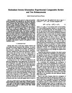
Figure 6: Graph showing the number of iterations required by CCD to reach the target, compared to the original distance of the hand to the target. chain, it is possible that some targets even within the radius of the chain are unreachable. We record the number of iterations required by the CCD method to either reach the target or to reach a stable position. For both methods we record how closely the target is reached and the sum of the joint angles as cost C.
5
Results
8.27% of targets were outside the radius of the chain. A further 2.23% were unreachable by the constrained chain. CCD reached 92.97% of all reachable targets when constrained within 20 iterations, with a mean number of 8.727 iterations. When unconstrained it reached 92.12% of the targets within 20 iterations with a mean of 8.351. Note that the mean also does not include those targets that were unreachable. As can be seen in figure 6, the number of iterations increases exponentially with the original distance of the end-effector to the target. The original angle of the target vector to the chain is also significant. As it increases so does the number of iterations. Triangulation reached each target on the first iteration as expected. The average cost of CCD using the unconstrained chain was 315.5o , compared to 173.9o when using the constrained chain. The triangular method when unconstrained had a mean cost of 159.9o ; When constrained this value was 141.5o .
6
Discussion
Every target that could theoretically be reached was reached by both algorithms, as expected. It is interesting to note that the constrained version of CCD performed slightly faster than the unconstrained version. There are several reasons for this:
Figure 7: 5-Jointed kinematic chain reaching for a close target. • The constraints prevented the chain from ’rolling in’ on itself as shown in figure 2. Thus the chain did not have to unroll itself before reaching the target. • The constrained chain had fewer but longer joints than the unconstrained chain. Thus the rotation of each joint had more of an effect on the remaining chain, especially in later iterations. As can be seen in figure 7, triangulation achieved more natural poses when reaching for the same target as CCD in figure 2. This is caused by the major joints rotating before the joints close to the end-effector. It is also worth noticing that most joints simply remain straight, instead of twisting in several different directions. This had an effect on the cost function, which was lower for the triangular method than for CCD using both kinematic chains. We can compare the complexity of the two algorithms using the number of calculations required for each joint. The dot product of two vectors in three-dimensional space requires three multiplications to compute. The cross product needs six multiplications. Solving the cosine equation as shown in equation 5 needs 5 multiplications and one division. This is approximately as complicated as a cross product. We define the number of calculations required for the rotation or transormation as r. If we label the number of calculations required for a dot product n, then both the cross product and the cosine equation both require 2n calculations. We can represent these values by the following equations:
NCCD = numIter ∗ numJoints ∗ (n + 2n + r) (9)
NT riangulation = numJoints∗(n+2n+2n+r) (10) Clearly NCCD > NT riangulation , when CCD requires more than one iteration. If we compare this with our data, then for the unconstrained chain we have a mean number of 8.351 ∗ 5 ∗ (3n + r) = 125.265n + 41.755r calculations using CCD, compared to 5 ∗ (5n + r) = 25n + 5r calculations using triangulation. Obviously our method requires significantly fewer calculations, and is thus faster to implement than CCD.
7
Future Work
Our implementation of the triangular method has only been for kinematic chains with one end-effector. If this algorithm were to be modified into a form that could find solutions for several end effectors, it could be used for more complex character models. The algorithm as it stands cannot accept constrictions on the axis of rotation. Both in character animation and robotics these restrictions often exist. Thus our method needs to be adapted to also accept these restrictions. Modifying the algorithm, by changing δb to 90o instead of 180o when a triangle cannot be formed, should also be investigated. This alternative might reduce the cost further, especially for constrained joints.
8
Conclusion
In this paper we have presented a novel method of solving the inverse kinematics problem. This new method, which is guaranteed to find a solution when it is available, is not iterative, therefore making it possible to predict the number of calculations required to reach a target. Like methods using the Jacobian Matrix the algorithm will find a solution immediately, instead of converging on a solution after several iterations. Yet unlike these methods it can deal with singularities as it does not require the Jacobian Matrix for its calculations. Our experiment shows that the triangular method requires on average many fewer calculations than CCD, both with constrained and unconstrained kinematic chains. At the same time it is just as accurate, finding a solution every time CCD does. Thus the triangulation method combines the best of both worlds. It is computationally cheaper than
CCD, yet just as accurate as algorithms calculating the Jacobian inverse or transpose of an inverse kinematics problem. Using a cost function we could show that it consistently requires less rotations than CCD, yet it is worth noting that our method does not guarantee optimal rotations (where each joint moves by a minimal amount); Like CCD it calculates angles one joint at a time, thus it is not possible for it to find such a minimal solution for the entire kinematic chain.
References [1] K. C. Gupta and K. Kazerounian, “Improved numerical solutions of inverse kinematics of robots,” in Proceedings of the 1985 IEEE International Conference on Robotics and Automation, vol. 2, pp. 743–748, March 1985. [2] A. Goldenberg, B. Benhabib, and “A complete generalized solution verse kinematics of robots,” IEEE Robotics and Automation, vol. 1, March 1985.
R. Fenton, to the inJournal of pp. 14–20,
[3] V. J. Lumelsky, “Iterative coordinate transformation procedure for one class of robots,” IEEE Transactions on Systems Man and Cybernetics, vol. 14, pp. 500–505, June 1984. [4] V. D. Tourassis and J. Ang, M.H., “A modular architecture for inverse robot kinematics,” IEEE Transactions on Robotics and Automation, vol. 5, pp. 555–568, October 1989. [5] M. Fedor, “Application of inverse kinematics for skeleton manipulation in real-time,” in SCCG ’03: Proceedings of the 19th spring conference on Computer graphics, (New York, NY, USA), pp. 203–212, ACM Press, 2003. [6] D. L. Pieper, The kinematics of manipulators under computer control. PhD thesis, Stanford University Department of Computer Science, October 1968. [7] J. Lander, “Making kine more flexible,” Game Developer, vol. 1, pp. 15–22, November 1998. [8] A. Canutescu and R. Dunbrack, Jr., “Cyclic coordinate descent: A robotics algorithm for protein loop closure,” Protein Science, vol. 12, pp. 963–972, May 2003. [9] L.-C. T. Wang and C. C. Chen, “A combined optimization method for solving the inverse kinematics problems of mechanical manipulators,” IEEE Transactions on Robotics and Automation, vol. 7, pp. 489–499, August 1991.