Neural network post-processing of grayscale optical correlator Thomas T. Lu 1a, Casey L. Hughlettb, Hanying Zhoua, Tien-Hsin Chaoa, Jay C. Hananc Jet Propulsion Laboratory/California Institute of Technology, 4800 Oak Grove Dr. M/S 303-300, Pasadena CA 91109; bZion Labs, Edmond, OK; cOklahoma State University, Tulsa, OK
a
ABSTRACT In real-world pattern recognition applications, multiple correlation filters can be synthesized to recognize broad variation of object classes, viewing angles, scale changes, and background clutters. Composite filters are used to reduce the number of filters needed for a particular target recognition task. Conventionally, the correlation peak is thresholded to determine if a target is present. Due to the complexity of the objects and the unpredictability of the environment, false positive or false negative identification often occur. In this paper we present the use of a radial basis function neural network (RBFNN) as a post-processor to assist the optical correlator to identify the objects and to reject false alarms. Image plane features near the correlation peaks are extracted and fed to the neural network for analysis. The approach is capable of handling large number of object variations and filter sets. Preliminary experimental results are presented and the performance is analyzed.
Keywords: pattern recognition, neural network, grayscale optical correlator.
1. INTRODUCTION Human beings are capable of recognizing objects and understanding images easily. However, a computer or a robot has a hard time to recognizing even a simple object in an unknown environment. The computer must be taught every possible view of the object as well as the environmental changes, in order to avoid confusion. In 3D space, an object has many variations in viewing angles, scale, rotation, sun angle, etc. It is almost impossible to teach the computer to remember all possible variations of a 3D object in 2D image form, not to mention the changing environment. In the past, many invariant algorithms have been proposed to reduce the dimensional complexity of the pattern recognition tasks. To name a few, Fourier transform (shift invariant), Mellon transform (scale invariant), circular harmonic transform (rotation invariant), and Hu moments, etc 1 - 6. Each algorithm reduces certain dimensional complexity, but imposes specific restrictions and may add other complexities. So far, there is not an algorithm that can match human performance. When a camera takes an image of a scene, the camera orientation can be recorded in the image file and transferred to the processor. The camera information contains the camera angles, magnification, and the time of the day, etc. The time of day information can be translated to the Sun angles. It determines the shadow length and the direction of the objects in the image. Assume the object is situated in a flat plane, then we can also estimate the shadow length, roll, and the pitch angles of the objects. This information reduces the dimensional requirement of the pattern recognition task. The possible yaw angles of the object can be from 0 to 360 degrees. Thus, a set of filters are needed to cover these yaw angles. In this paper, a pattern recognition process is presented that uses OT-MACH (optimum trade-off Maximum Average Correlation Height) based filters to construct a filter bank of 3D objects. Variations of the scale, yaw, pitch, and roll of the objects are built into the composite filters, which form a filter bank. A gray scale optical correlator (GOC) is used to load the filters from the filter bank rapidly and identifies the objects in a unknown image. A neural network is trained as a post processing step to confirm the identification and eliminate false alarms of the GOC system.
1
e-mail:
[email protected] , Tel: (818) 393-2981, Fax: (818) 393-4272
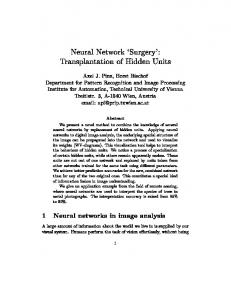
2. SYSTEM ARCHITECTURE JPL has developed a software tool set that generates the OT-MACH filters, performs the simulation of the optical correlation and evaluates the results 7 – 9. The procedures are as follows (See Figure 1 for illustration): The camera information is extracted and sent to the object model bank. The object model bank contains the 3D models of the objects. It produces a set of training images of the objects of interest. The training images contain various object scale and orientations that could be seen from the particular camera angle. The training images are sent to the OT-MACH filter generator to generate a set of filters. The software performs the optimization of filter training parameters. A set of neurons are also trained using the object images and the correlation outputs. The filters and the neurons are generated on-line. They are fed into the GOC and RBFNN simulators for pattern recognition operations. The input image is preprocessed and segmented to 512x512 pixel sizes, and then fed to the GOC simulator. A series of correlation operations are performed on the image by a set of filters. The correlation outputs are analyzed by the PSR method. The peaks with PSR and peak values above a set threshold will be further evaluated by the neural network post-processor. The RBFNN is used to evaluate the features in each peak location and classify them into two categories: object confirmed, or false alarm rejected.
Training Images
Training Images
Camera Info
Object Model Bank
OT-MACH Filter Generation
Input Image
Filter Set Segmented Images Preprocessing
Optical Correlator
RBFNN Training
Neuron Update RBF Neural Network
Object Recognition
Figure 1: Architecture of an optical correlator and neural network pattern recognition system
In the following sections, the functions of the system are discussed in detail.
3. GRAY SCALE OPTICAL CORRELATOR (GOC) SYSTEM JPL has developed a compact gray scale optical correlator 7. It is capable of 1000 frames per second parallel correlation operations on 512 x 512 pixel images. Figure 2 shows the compact GOC module. The size of the GOC is only 2” x 2” x 6”.
(a)
(b)
Figure 2: A compact grayscale optical correlator (GOC) module: (a) top view, (b) side view.
4. OT-MACH FILTER GENERATION 4.1 OT-MACH Filter Overview The OT-MACH (optimum trade-off Maximum Average Correlation Height) is an Fourier transform (FT)-based algorithm 10 -13. It is formulated for the optimal implementation on an optical correlator. The OT-MACH filter algorithm balances simultaneously several conflicting performance measures such as Average Correlation Height (ACH), Average Similarity Measure (ASM), Average Correlation Energy (ACE) and Output Noise Variance (ONV), by minimizing the following energy function:
E (h ) = α (ONV ) + β ( ACE ) + γ ( ASM ) − δ ( ACH ) = αh + Ch + βh + D xh + γh + S xh − δ hT m x
(1)
The resulting OT- MACH filter (in frequency domain) is given by 10 - 11
h =
M x α C + β D x + γS x
(2)
where α, β and γ are nonnegative parameters. Mx is the average of the training image vectors Xi, i=1, …, N. C and Dx are the diagonal power spectral density matrices of additive input noise and of the training images, respectively. Sx is the similarity matrix of the training images: N
Sx = ∑ i =1
(X i − M x )2 N
(3)
By choosing different values of α, β and γ, one can control the OT-MACH filter's behavior to suit different application requirements. For example, when α is increased, the resulting filter has relative good noise tolerance but broad peaks. If
β is high, then the filter generally gives sharp peaks and good clutter suppression but is more sensitive to distortion. By increasing γ value, the filter is designed with high tolerance for distortion. In many ATR applications a target is embedded in a cluttered background. The adjustment of the parameters gives added flexibility to optimum filter design. We have developed a Windows based program to perform optimal search of the α, β and γ values. 8, 9
4. 2 Correlation Operations The input image is cut into 512 x 512 pixels in size. It is Fourier transformed into the spectral domain. It is then multiplied by the filter and inverse Fourier transformed to the correlation plane.
C(u,v) = F -1{F {I(x,y)}H(ω,ξ)},
(4)
Where C(u,v) is the correlation plane image, I(x,y) the input image, F and F -1 stand for the Fourier and the inverse Fourier transforms, respectively, and H(ω,ξ) is an OT-MACH filter.
4. 3 Filter Bank Generation Using above OT-MACH filter algorithm one can generate distortion tolerant composite filters. FFT-based filters are shift invariant, but they are still sensitive to scale, rotation, perspective, and lighting conditions. In addition, targets may also be partially occluded, camouflaged or may be decoys. In order to achieve the highest level of assurance that the targets are identified with minimal errors while the number of filters is reasonably small, all desired variations and distortions in targets need to be carefully included systematically when generating filters. A filter bank is generated for the targets in which every filter covers a small range of variations, and a set of filters covers the full expected range of those variations. We have developed a software tool to streamline the filter synthesis/testing procedure effectively while maintaining filter performance. In order to cover all potential target perspectives with up to 6-degree-of-freedom, a large bank of composite filters have to be generated. The filter training images can be either obtained from real-world examples or from a 3D synthesizer. Figure 3 shows a sub-set of the example training images in changing rotation angles. The corresponding OT-MACH filter is shown in Figure 4.
Figure 3: A set of training images for composite filter synthesis
It may take well over 1000 filters to cover a range of aspect and scale changes of an object. Filter bank management software is needed to keep track of the filters and update the filter bank after new filters are generated.
Figure 4: An example of the OT-MACH filter
5. RADIAL BASIS FUNCTION NEURAL NETWORK (RBFNN) JPL has been developing neural network algorithms and their hardware implementation 17, 20 - 22. A neural network has the characteristics of emulating the behavior of a biological nervous system and draws upon the analogies of adaptive biological learning. Because of their adaptive pattern classification paradigm, they possess the significant advantages of a complex learning capability plus a very high fault tolerance. They are not only highly resistant to aberrations in input data, but they are also excellent at solving problems too complex for conventional technologies such as rule based and determinative algorithm methods. A unique contribution of neural networks is that they solve many of the obstacles experienced with conventional algorithms. JPL has recently been investigating a real-time trainable digital neural network -- Radial Basis Function neural network (RBFNN) paradigm. This RBFNN model can be easily implemented in customized semiconductor hardware using the FPGA (Field Programmable Gate Array) technology. This neural network hardware is a unique digital processor that is capable of performing all neural training and classification operations including matrix-matrix multiplications, synapse weight computations and thresholding functions dictated by the RBF neural paradigm.17 5.1 Radial Basis Function Model The post-processing algorithm is based on an adaptive RBFNN architecture. RBFNN algorithms have advantages for pattern recognition, including practical implementation in parallel hardware for real-time operation, sparse data representation for low power, and fast learning for mapping of the input space 18, 19. A software simulation of an adaptive RBFNN object tracker has been implemented. The RBFNN algorithm consists of mapping an N-dimensional feature space by prototypes (training examples). Each prototype is a vector representing a position in the feature space, and is represented by a neuron with a receptive field representing a local region of space around the prototype center where generalization is possible. The recognition task then consists of evaluating if a new input feature vector lies within the influence field of any neuron stored in the network. Fast learning in the RBF lends itself to real-time adaptation to changing target features when objects are viewed from varying angles and the imagery changes scale with distance. The Radial Basis Function (RBF) neural network learns 'by example' from data samples and corresponding categories. A block diagram of this system is shown in Figure 5. Feature extraction methods are designed to tailor a specific class of targets. These feature vectors, representing the target of interest, are then fed into the neural network processor. A gradient feature extractor may be suited for detecting the edges of an object:
F ( x, y ) = ∑ x
∂I ( x, y ) ∂I ( x, y ) +∑ , ∂y ∂x y
(5)
Where I(x, y) is the input pixel value at (x, y).
RBF Neural Network Input Image
Feature ID Feature Extractors
On-Line Learning Figure 5: Functional block diagram of a Radial Basis Function neural network (RBFNN).
A neuron distance is calculated from each neuron to the input feature:
D(N) = |Wn(x, y) – F(x, y)|,
(6)
Where Wn (x, y) is the Nth neuron weight vector. If the input feature vector falls within the influence field of a neuron, then it is classified as belonging to this neuron class. The influence field of a neuron is a multi-dimensional hyper-spherical area centered from the neuron. The radial distance between the center and the edge of the influence field is defined by the shortest distance between the neuron and the counter examples of a different class or clutters, as shown in Figure 6. Each neuron adjusts its influence fields when presented with examples of objects and clutters so that it occupies as large an area as possible, but not to collide with counter examples. The influence field is defined as
Inf(N) = min(Dce(N)),
(7)
Where Dce (N) is the distance between counter-examples and the Nth neuron. By presenting proper objects and counter examples, the influence fields of the neurons are fine tuned to define a proper non-linear boundary. Background clutters can be used as the counter examples. Shifting the window around the object area, then extracting the features from the windows also serves as good counter examples.20 Eventually, the influence fields of the neurons occupy all feature space belong to the objects, setting the non-linear boundary between the objects and the counter examples and clutters, as shown in Figure 7.
Counter Examples Old Influence Field
New Influence Field Neuron
Feature Space
Figure 6: Influence field of a neuron and counter examples.
Feature 2 Influence Fields
0
Feature 1
Figure 7: An example of RBFNN in a simplified 2-D feature space. By presenting proper objects and counter examples, the RBFNN forms a non-linear boundary between the features of the objects and the clutters.
6. SIMULATION RESULTS A set of training object images were extracted from the 3D models. The sampling interval is 5 degrees angular and 7% scale. For a given input image, based on its camera information, a set of 24 filters are generated to cover 15 degree roll and pitch angle variation and 360 degree yaw angle. The objects are embedded in arbitrary background images. The intensity of the image areas varies dramatically to simulate the climate variation and urban changes. Figure 8(a) shows an image with an embedded object. Figure 8(b) shows the correlation plane. The peaks are located in the object coordinates, indicating the detection of the objects. However, some clutters also cause false peaks in the correlation plane. A peak to side lobe ratio (PSR) method can increase the reliability of the correlation detection. However, due to the complexity of the background clutters, further post processing is needed to eliminate the clutters.
Positive Targets
(a)
(b)
Figure 8: (a) An input image with objects embedded, and (b) the correlation plane show the detection of the object and the false alarm of the clutters.
A RBFNN is used to train with the object features. Figure 9 shows an example of the gradient features extracted from the targets and non-targets. The gradient features capture the edge information of a generally rectangular shaped object. The relative locations, magnitudes and the signs of the edges are shown as the peaks of the feature vectors. The clutters show random patterns in the gradient feature vectors. The object features are used to train the neural net. The clutter features are used as the counter examples of the neural net training. The RBFNN is then used to examine the content of each peak location in the correlation plane. In the preliminary experiments, over 60% of the false alarms are eliminated by the RBFNN. From initial experiment results, we can see the RBFNN is capable of reducing false alarms significantly from the correlation results. We are fine tuning the RBFNN as a post-processor to increase the sensitivity and reliability of the optical correlator.
Figure 9: Examples of the target and non-target gradient features for the RBFNN.
7. CONCLUSIONS Initial results of combining the software simulation tools of the OT-MACH filter generation and the RBFNN training confirm a reduction of the false alarm rate for automatic target recognition. The procedure of generating a filter bank to cover angular and scale variations of the object in 3D views has been discussed. An improvement of the specificity of optical correlation was shown through advanced training of the image features using new tools, and object gradient features were reported. Additional research is underway to optimize the neural network training of the object features further improving the reliability of the pattern recognition processes.
8. ACKNOWLEDGEMENTS The research described in this paper was carried out by the Jet Propulsion Laboratory, California Institute of Technology, under a contract with the National Aeronautics and Space Administration.
9. REFERENCES 1. 2.
D. Casasent, D. Psaltis, "New optical transforms for pattern recognition," Proc. IEEE 65, 77-84, 1977. Y. Yang, Y. N. Hsu, and H. H. Arsenault, "Optimum circular filters and their uses in optical pattern recognition," Opt. Acta 29, 627-644, 1982.
3. 4. 5. 6. 7. 8. 9. 10. 11. 12. 13. 14. 15. 16. 17. 18.
19.
G. F. Schils, D. W. Sweeney, "Rotationally invariant correlation filtering," J. Opt. Soc. Am. A 2, 1411-1418, 1985. D. Casasent, M. Krauss, "Polar camera for space-variant pattern recognition," Appl. Opt. 17, 1559-1561, 1978. H. J. Caulfield, M. H. Weinberg, "Computer recognition of 2-D patterns using generalized matched filters," Appl. Opt. 21, 1699-1704, 1982. J. Riggins, S. Butler, "Simulation of synthetic discriminant function optical implementation," Opt. Eng. 23, 721726, 1984. T-H. Chao, G. Reyes, Y. Park, "Grayscale Optical Correlator", SPIE v.3386, 1998. H. Zhou, C. L. Hughlett, J. C. Hanan, T. Lu, T-H. Chao. “Development of streamlined OT-MACH-based ATR algorithm for grayscale optical correlator,” p. 78-83, Optical Pattern Recognition XVI; SPIE 5816 , 2005. J. C. Hanan, C. L. Hughlett, H. Zhou, T.-H. Chao, “Grayscale Optical Correlator Work Bench” NASA NTR41021, 2004. J. C. Hanan, C. L. Hughlett, T.-H. Chao, “Radial Basis Function Neural Network Tracker.” NASA NTR-40071 , 2003. T.-H. Chao, G. Reyes, H. Zhou, "Automatic Target Recognition Field Demo Using a Grayscale Optical Correlator", SPIE v.3715, p.399-406, 1999 T.-H. Chao, H. Zhou, G. Reyes, "Compact 512x512 Grayscale Optical Correlator", SPIE v.4734, p.9-12, 2002. B. V. K. Vijaya Kumar, D. Carlson, A. Mahalanobis, "Optimal trade-off synthetic discriminant function filters for arbitrary devices," Opt. Lett. 19, pp.1556-1558, 1994. H. Zhou, T.-H. Chao, "MACH Filter Synthesizing for Detecting Targets in Cluttered Environment for Grayscale Optical Correlator," SPIE 3715, pp. 394-398, 1999. H. Zhou, T.-H. Chao, G. Reyes, "Practical saturated filter for grayscale optical correlator using bipolaramplitude SLM," SPIE 4043, 2000. H. Zhou, T.-H. Chao, B. Martin, N. Villaume, "Simulation of miniature optical correlator for future generation of spacecraft precision landing," SPIE 5106, p.179-185, 2003. J. C. Hanan, T.-H. Chao, P. Moreels, “Neural network tracking and extension of positive tracking periods”, SPIE, Optical Pattern Recognition XV, 2004. F. Yang, M. Paindavoine, “Implementation of an RBF neural network on embedded systems: Real-time face tracking and identity verification”, Special Issue on Hardware Implementations, IEEE Trans Neural Networks 14(5):1162-1175, 2003. Acosta FMA, “Radial basis function and related models – an overview”, Signal Processing 45(1):37-58, 1995.
20. J. C. Hanan, C. L. Hughlett, T.-H. Chao, “Radial Basis Function Neural Network Tracker.” NASA NTR-40071 , 2003. 21. J. C. Hanan, H. Zhou, T.-H. Chao, “Precision of a radial basis function neural network tracking method,” SPIE, Optical Pattern Recognition XIV, 5106, 146-153 , 2003. 22. J. C. Hanan, T.-H. Chao, C. Assad, C. L. Hughlett, H. Zhou, T. Lu, “Closed-Loop Automatic Target Recognition and Monitoring System,” p. 244-251, Optical Pattern Recognition XVI; SPIE 5816 , 2005.