unstructured light field rendering using on-the-fly

UNSTRUCTURED LIGHT FIELD RENDERING USING ON-THE-FLY FOCUS MEASUREMENT

Keita TAKAHASHI

Takeshi NAEMURA

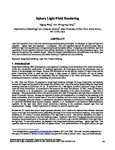
School of Information Science and Technology, the University of Tokyo 7-3-1, Hongo, Bunkyo-ku, Tokyo, 113-8656, Japan {keita,naemura}@hc.ic.i.u-tokyo.ac.jp ABSTRACT This paper introduces a novel image-based rendering method which uses inputs from unstructured cameras and synthesizes free-viewpoint images of high quality. Our method uses a set of depth layers in order to deal with scenes with large depth ranges. To each pixel on the synthesized image, the optimal depth layer is assigned automatically based on the on-the-fly focus measurement algorithm that we propose. We implemented this method efficiently on a PC and achieved nearly interactive frame-rates. 1. INTRODUCTION Image-based rendering (IBR) means a group of techniques for synthesizing free-viewpoint images from a set of preacquired images. Compared with conventional graphics techniques based on geometric primitives, IBR methods can produce highly photo-realistic images with less computation cost. Due to this advantage, IBR is used for live 3D video systems [5, 10, 11, 12], and expected as a key technology in telecommunication and virtual reality systems. In practical cases, we have to use a structure model as well as images in order to keep the needed number of images at a reasonable level (the theoretical analysis is given in [1]). This paper introduces an IBR method which uses a set of depth layers. When rendering an image using depth layers, we should assign the optimal layer to each pixel on the image. In contrast to some prior works which use depth layers [2, 7, 9], our method does not need any pre-processing step for shape/depth estimation. In our method, depth assignment is completed by an on-the-fly process which we call the focus measurement. In [8], we have already proposed a focus measurement method which is used for light field rendering. But the application scope was limited to structured inputs, where input cameras should be aligned in parallel at constant intervals. This paper extends the application scope of the prior method to more generalized inputs by redefining the focus measurement algorithm in the spatial domain. Since the proposed method can deal with unstructured inputs, we call it “unstructured light field rendering using on-the-fly focus measurement”. We also report an efficient implementation of

0-7803-9332-5/05/$20.00 ©2005 IEEE

our method on a PC, which enables rendering at nearly interactive frame-rates. 2. ALGORITHM Suppose that input images are captured by multiple cameras which are located roughly on a plane. We consider a practical scenario where input cameras are not exactly aligned, but calibrated in advance. Our goal is to synthesize freeviewpoint images from images by those cameras. We use a set of depth layers for synthesizing images. Let N be the number of layers, and zn be the depth of the n-th layer. Our algorithm consists of the following 3 steps, all of which are on-the-fly operations for each frame. 1. N images, in which the n-th image corresponds to the n-th plane of the layers, are synthesized. 2. We detect in-focus parts on those synthesized images by the focus measurement. 3. Those detected parts are integrated into the final image. The remainder of this section describes these steps in detail. 2.1. Rendering for Each Plane Figure 1 shows the configuration. Though the sysmtem is configured in the 3-D space in practice, we reduce the dimension to 2-D for simplicity of explanation. Suppose that we synthesize an image at the rendering camera. Ci denotes the i-th input camera, and Pi denotes the projected position of its center on the plane model. In order to synthesize an image at the rendering camera, all light-rays which pass through the projection center of the rendering camera need to be gathered. Suppose a case where we obtain the color of the light-ray represented by r in Fig. 1. Let P be the intersection point of r and the plane model. We read out the light rays (ri (P) and ri+1 (P)) from the two nearest cameras (Ci and Ci+1 ) which pass through P. The color of r is obtained as follows: color(r) = (1 − t) · color(ri (P)) + t · color(ri+1 (P)). (1) where the point P divides the segment Pi Pi+1 internally in the ratio of t : 1 − t. Note that this method itself is not a new one, since it is one of the simplest cases described in [3, 4]. The important

Pi

Pi+1

P

t

1-t

ri (P)

object 2

object 2 plane model ( Z = zi )

object 1

object 1

ri+1 (P)

Ci

Ci+1

r

Ci+1

Ci (Z=0)

r(1)

Ci+2

r(2)

Ci r(1)

base mode rendering camera

Fig. 1. The basic configuration. point is that in the synthesized images by this plane model, objects near the model are clear and sharp (in-focus), but objects apart from it are blurred and ghosted (out-of-focus) (See Fig. 3(a)–(c)). That is why we need multiple depth layers (step 2 and 3 operations) in order to make the whole scene in-focus in the final synthetic image. 2.2. Focus Measure The next step is to calculate focus measure values for detecting in-focus parts. In our prior work [8], we constructed a focus measurement algorithm in the frequency domain based on the sampling theorem [1]. But due to the nature of the sampling theorem, the scope of discussion was limited to regularly structured inputs, i.e. cameras should be aligned in parallel at constant intervals. In this paper, we reconstruct the focus measurement algorithm in the spatial domain in order to apply it to unstructured inputs directly. Suppose that two images are synthesized by the two modes shown in Fig. 2 for an identical viewpoint. The base mode shown on the left uses all of the input cameras for rendering (it is the normal case), while the reference mode shown on the right uses a subset of it, in which input cameras are skipped alternately. Both modes uses Equation (1) for synthesizing each light-ray. The dotted lines show the light-rays used for synthesizing r(1) and r(2). In both modes, the plane model is situated at the depth of Object 1. Therefore, Object 1 is in-focus, but Object 2 is out-of-focus. Assume that non-diffusive reflections and occlusions are negligible. The light-ray r(1), which is emitted from an in-focus point, is synthesized to have one identical color in both modes. This is because both modes use such lightrays that are emitted from one identical point on the object surface for synthesizing r(1). On the other hand, the light-

Ci+1

Ci+2

r(2)

reference mode

Fig. 2. Two synthesis mode for the focus measurement. ray r(2) (emited from an out-of-focus point) could have different colors according to the mode. Consequently, in the synthesized images by the two modes, in-focus parts are to be synthesized identically, while out-of-focus parts would show some differences. This nature can be used for detecting in-focus parts. According to the above discussion, we propose a focus measure for detecting in-focus parts. Let In (x, y) and Rn (x, y) be the synthesized images with the plane model at zn by the base mode and the reference mode, respectively. The focus measure value fn at a pixel (x, y) is defined as follows: subn (x, y) = |In (x, y) − Rn (x, y)| (2) X X subn (x + k, y + l) fn (x, y) = . (3) (2M + 1)2 −M ≤k≤M −M ≤l≤M

where M denotes a positive integer. When fn (x, y) is small enough for a pixel (x, y), the pixel is regarded to be infocus in In (x, y). Equation (3) is a smoothing operation for reducing the uncertainty of detecting out-of-focus parts as in-focus parts. A more popular way for evaluating the depth-correctness is to compare the color of coresponding pixels on the input images [6]. Zhang and Chen [12] incorporated this scheme into their real-time IBR system by limiting the evaluation to the selected points (vertices of the mesh model) on the synthesized image. In contrast, our method evaluates the synthesized light-rays (pixels on the synthesized image), and achieves per-pixel depth evaluation in real-time. 2.3. Final Image Synthesis When focus measure values fn (x, y) have been calculated for all zn , the remaining process is straightforward. The index of the optimal depth no for a pixel (x, y) is given by

minimum search of fn as follows: no (x, y) = arg min (fn (x, y)) . n

(4)

Then, In (x, y) (n = 1, .., N ) are selectively integrated into a final image I(x, y) based on no (x, y). I(x, y) = Ino (x,y) (x, y).

(5)

our environment. Then, synthesized images are transferred to the main memory for the following operations. The next stage (stage B) is to calculate focus measure values for all n. In order to reduce the computation cost, we reorganize Equation (3), whose computation order is O(M 2 ), into the recurrence equation as follows (O(M )): fn (x, y) = fn (x − 1, y) +

3. IMPLEMENTATION We implemented our algorithm on a Pentium 4 3.2 GHz PC with 2.0 GB main memory. The graphics card has a NVIDIA GeForce 5800 processor and 128 MB video memory built in. We developed software with C and OpenGL. In order to stabilize the focus measurement, we use 4 reference modes which correspond to the combination of the skipped lines (odd/even rows and odd/even columns) on the input camera array. We use the following equation for calculating subn instead of Equation (2). X subn (x, y) = |In (x, y) − Rnj (x, y)|. (20 ) j

where Rnj (x, y) denotes the synthetic image by the j-th reference mode with a plane model at zn . Therefore, the pseudocode is as follows: for (novel viewpoint){ /* Stage A: synthesize N images by each mode */ for (n := 1 → N ){ Synthesize In (x, y); for (j :=1 → 4) Synthesize Rnj (x, y); } /* Stage B: calculate focus measure values */ for (n := 1 → N ){ Calculate subn (x, y); /* by Equation (20 ) */ Calculate fn (x, y); /* by Equation (3) */ } /* Stage C: synthesize the final image */ Calculate z(x, y); /* by Equation (4) */ Calculate I(x, y); /* by Equation (5) */ } At the first stage (stage A), we synthesize multiple images (N images by each mode) with plane models. We conduct this process on the graphics hardware using multitexturing technology similarly to [3]. In this process, each input image is modulated by the aperture texture and projected onto the plane model using the projective texture coordinate. The aperture texture corresponds to the pattern of contribution of each image on the plane model. The projective texture coordinate is derived from the calibration data of each camera, and ensures perspective-correct mapping of the texture. Accelerated by the graphics hardware functions, this process runs at more than 1000 times/second in

X subn (x + M, y + l) (2M + 1)2

−M ≤l≤M

−

X subn (x − M − 1, y + l) . (2M + 1)2

(30 )

−M ≤l≤M

In our implementation, the stages A and B would occupy the most part of the total processing time. However, these stages can be partially parallelized: for example, calculation of sub1 and f1 can be started at the point where I1 and R1j have been synthesized and reached to the main memory. Thanks to Hyper-Threading Technogy which is available on the Pentium CPU, we could reduce the total compuation time by implementing these stages in multi-threads. 4. EXPERIMENTS As the input, we use multi-view image data provided by Advanced Multimedia Processing Laboratory of Carnegie Mellon University 1 . These images are captured by 48 (6 rows by 8 columns) calibrated cameras with 320 × 240 pixels. Though these cameras are located roughly on a plane, they are not evenly spaced, nor facing the same direction. Therefore, it is a good example of unstructured inputs. We set the size of synthetic images to 320 × 240 pixels, the number of layers (N) to 7, and M = 5 in Equation (3). Shown in Fig. 3 is the synthesis process at a certain viewpoint. Figure 3 (a), (b), and (c) are synthesized with a single-plane model at z2 , z5 , and z7 , respectively (the depth indexes are assigned in far-to-near order). In these images, strong focusing effects are observed: out-of-focus parts are severely damaged. One of the reference images at z7 is shown in Fig. 3 (d). As discussed in 2.2, in-focus parts are identical in Fig. 3 (c) and (d), while out-of-focus parts are different. Therefore, as shown in Fig. 3 (e), the subtraction between the base image and the references is used for detecting in-focus parts. Note that textureless regions (for example, the background) could be detected as in-focus regions at any depth, but it does not affect the quality of the final synthetic images. Shown in Fig. 3 (f) is the final allin-focus image. We can synthesize all-in-focus images for arbitrary viewpoints as shown in Fig. 4. Figure 5 shows the processing time for each stage. By parallelizing the stages A and B, we have reduced the total processing time about 24 %. Though much more speeding up is desired, we have achieved nearly interactive framerates (7.4 fps) at present. 1 http://amp.ece.cmu.edu/projects/MobileCamArray/

(a) I2 (x, y)

(b) I5 (x, y)

(c) I7 (x, y)

(d) R7 (x, y)

(e) sub7 (x, y)

(f) I(x, y) (final image)

Fig. 3. Synthesis process at a certain viewpoint: (a)–(c) synthesized images with a single-plane model at different depths, (d) a reference image at z7 , (e) the subtraction image at z7 , (f) the all-in-focus image. 5. CONCLUSIONS In this paper, we proposed a novel IBR method that uses inputs from unstructured cameras and synthesizes freeviewpoint images using a set of depth layers. Without any pre-processing for shape/depth reconstruction, our method conducts pixel-by-pixel depth assignment using the on-thefly focus measurement. We also reported an implementation and some experimental results for showing the effectiveness of our method. Our future work will be focused on speeding up of our method and its application to dynamic scenes and live 3D video systems like [5, 10, 11, 12]. Acknowledgement: One of the authors, K. Takahashi is a Research Fellow of the Japan Society for the Promotion of Science. Special thanks go to Prof. H. Harashima of the University of Tokyo for helpful discussions.

6. REFERENCES [1] J. -X. Chai et al., “Plenoptic sampling,” Proc. ACM SIGGRAPH 2000, pp. 307–318, 2000. [2] A. Isaksen et al., “Dynamically reparameterized light fields,” MIT-LCS-TR-778, 1999. [3] A. Isaksen et al., “Dynamically reparameterized light fields,” Proc. ACM SIGGRAPH 2000, pp. 297–306, 2000. [4] M. Levoy and P. Hanrahan, “Light field rendering,” Proc. ACM SIGGRAPH 96, pp. 31–42, 1996. [5] T. Naemura et al., “Real-time video based modeling and rendering of 3D scenes,” IEEE CG&A, 22, 2, pp. 66–73, 2002. [6] S. Seitz and C. Dyer, “Photorealistic scene reconstruction by voxel coloring,” IJCV, 25, 3, pp. 151–173, 1999. [7] J. Shade et al., “Layered Depth Images,” Proc. ACM SIGGRAPH 98, pp. 231–242, 1998.

Fig. 4. Synthesized results for other viewpoints. Stage C et al. non-parallelized

Stage B

Stage A Stage A + B

parallelized

0

50

5.7 fps 7.4 fps

100 150 processing time (msec)

200

Fig. 5. Processing time for each stage. [8] K. Takahashi et al., “A focus measure for light field rendering,” Proc. IEEE ICIP 2004, pp. 2475–2478, 2004. [9] X. Tong et al., “Layered lumigraph with LOD control,” J. Visualization & Computer Anim., 13, 4, pp. 249–261, 2002. [10] T. Yamamoto et al., “LIFLET: light field live with thousands of lenlets,” ACM SIGGRAPH 2004, etech 0130, 2004. [11] J. C. Yang et al., “A real-time distributed light field camera,” Proc. EGWR 2002, pp. 77–86, 2002. [12] C. Zhang and T. Chen, “A self-reconfigurable camera array,” Proc. EGSR 2004, pp. 243–254, 2004.