Fast (Spherical) Light Field Rendering with Per-Pixel Depth

TECHNICAL REPORT, COMPUTER GRAPHICS GROUP, UNIVERSITY OF SIEGEN, 2007

Fast (Spherical) Light Field Rendering with Per-Pixel Depth Severin Todt, Christof Rezk-Salama and Andreas Kolb Abstract— Image-based rendering techniques are a powerful alternative to traditional polygon-based computer graphics. This paper presents a novel light field rendering technique which performs per-pixel depth correction of rays for high-quality reconstruction. Our technique stores combined RGB and depth values in a parabolic 2D texture for every light field sample acquired at discrete positions on a uniformly sampled sphere. Image synthesis is implemented on the GPU as a fragment program which extracts the correct image information from adjacent cameras for each fragment by applying a per-pixel depth correction of rays. We show that the presented image-based rendering technique provides a significant improvement compared to previous approaches. We explain two different rendering implementations which make use of a uniformly sampled parameterisation to minimize disparity problems and ensure full six degrees of freedom for virtual view synthesis. While one rendering algorithm implements a run-time efficient iterative refinement approach for rendering light fields with per pixel depth correction the other approach employs a raycaster for per pixel depth correction and provides superior rendering quality at moderate frame rates. GPU based per-fragment depth correction of rays, used in both implementations, reduces ghosting artefacts to a non noticeable amount and provides a rendering technique that performs without exhaustive pre-processing for 3D object reconstruction or real-time ray-object intersection calculations at rendering time. Index Terms—Image-Based Rendering, Light Field.

✦ 1

I NTRODUCTION

Research in the field of image-based rendering (IBR) has contributed algorithms for real-time generation of photorealistic images of complex scenes. Generally, these algorithms are based on a collection of pre-acquired input images to produce new, virtual views. Unlike the polygonal rendering pipeline, IBR techniques are almost independent of scene complexity thus providing an efficient solution for photorealistic image synthesis at a predictable computational cost. The accuracy of continuous light field reconstruction can be improved if information about the scene geometry is taken into account. Depth information as well as polygonal approximations of the observed scene have been used for scene representation in a selection of IBR implementations to enhance image quality [7, 19, 23, 20, 3]. Depth estimation, however, has been identified to be crucial for the performance of rendering algorithms which apply depth correction of rays to improve image synthesis results. Vogelgsang et al. [22] have shown that best rendering performance can be achieved if depth determination can be reduced to a simple lookup, i.e. depth information which can be obtained directly from depth-maps. The approach described in this paper represents the result of our effort to develop an image-based scene representation that can directly take advantage of combined color and depth information for best rendering performance and image-synthesis quality. We present a new light field parameterisation and rendering algorithms based on a sparse set of discrete light field samples arranged on the surface of a camera sphere around an object in combination with associated per-pixel depth information. The spherical alignment ensures full 6 DOF for image synthesis of new virtual views and avoids disparity problems by using a uniformly sampled sphere. For highquality real-time reconstruction our advanced GPU-based rendering technique directly employs the full set of combined per pixel color and depth information acquired for every sample position. The remainder of the paper is structured as follows. In Section 2 we give an overview of relevant related work, including a survey on existing light field approaches. In Section 3 we introduce our light field representation and show the benefits with respect to combined RGB and depth data. Section 4 describes our novel techniques for GPU-based light field rendering with per-pixel depth refinement. In • Severin Todt, Christof Rezk-Salama and Andreas Kolb are with the Computer Graphics Group of the University of Siegen, Germany. E-mail: [email protected].

Section 5 we explain how light fields can be efficiently generated from 3D geometry. Section 6 evaluates the technique with respect to image quality and rendering performance. In Section 7 we draw conclusions and comment on future work. 2

R ELATED W ORK

The use of environment maps to capture the incoming light in a texture map [2, 8] has inspired several successive IBR techniques. As environment maps record the incident light arriving from all directions at a given point each individual environment map of a scene describes a concrete sample of the plenoptic function [15] as desribed by Adelson and Bergen [1]. The plenoptic function describes all of the radiant energy that can be received at a certain point in space (Vx ,Vy ,Vz ) from an arbitrary direction (θ , φ ) at a certain moment in time t for a chosen band of wavelengths λ :

ρ = P(θ , φ , λ ,Vx ,Vy ,Vz ,t)

(1)

Given a set of discrete samples of the plenoptic function, the goal of image-based rendering techniques is to generate a continuous representation of that function. Most IBR approaches reduce the 7D plenoptic function to a 5D plenoptic function by restricting it to a static lighting situation, eliminating t and reducing the wavelength λ using the primary values RGB. For objects being observed from positions either completely outside or completely inside its convex hull, the observation space can be assumed to be free of occluders. This assumption leads to further reduction of the plenoptic function by erasing spatial redundancies of the 5D plenoptic function. The plenoptic function can than be expressed as function on the space of oriented lines. The function of position and direction is described as light field [14]. Different discretisation methods for the 4D parameterisation lead to a variety of different IBR methods. Traditionally, image based rendering approaches are classified by the amount of geometric information being used for image synthesis. This classification leads to the IBR continuum introduced by Kang [12] and Lengyel [13]. Levoy and Hanrahan [14] use different criteria to categorize IBR techniques. These are the parameterisation and representation of the light field, the method to generate or acquire the light field and the approach to fast and accurate reconstruction of different views. Each of the techniques reviewed in the following section focuses on certain aspects of the above mentioned challenges. The individual approaches have influenced different parts of our work. Two Plane Light

TECHNICAL REPORT, COMPUTER GRAPHICS GROUP, UNIVERSITY OF SIEGEN, 2007

Field Rendering (see Section 2.1) introduces the 4D plenoptic function, Lumigraph Rendering (see Section 2.1) exploits geometric information for increased image quality and introduces full 6 DOF for virtual view synthesis and Spherical Light Field Rendering (see section 2.2) employs uniform spherical parameterisations to avoid disparity problems. Free Form Light Fields as well as Unstructured Lumigraphs are targeted at hand-held light field acquisition for non-uniform parameterisations, both of them applying depth correction for improved rendering quality. 2.1 Two-Plane Parameterisations Light field rendering as proposed in the original paper by Levoy and Hanrahan [14] restricts objects to lie within a convex cuboid bounded by two planes, the camera plane and the image plane. Rays describing the observation space are parameterised by their intersection points with these two planes leading to the 4D plenoptic function. A set of such two planes is called a light slab. Reconstruction of the light field for a ray described by the intersection points with the two planes (u, v,t, s) is performed by quadri-linear interpolation of the images taken by the cameras positioned around the intersection point on the camera plane(u, v). It has been shown that light field rendering as described above will provide satisfactory rendering results, if the observed object is positioned exactly on the image plane. In the general case, noticeable ghosting artefacts will appear due to incoherent light field information for adjacent rays. Incoherence results from rays hitting the object at a surface point far from the image plane, thus resulting in deviating intersection points on the image plane (see Figure 1). The Lumigraph introduced by Gortler et al. [7] uses a proximity polygonal object representation to overcome incoherence by applying a depth correction of the rays. With ray correction significant improvement in image quality for generated novel views can be achieved. Improved quality comes at the price of time consuming pre-processing steps to generate the proximity object. Lumigraph rendering performance is clearly limited by the depth estimation performance applied for ray correction. Discrete depth values are estimated by a computational expensive raycasting approach at rendering time. The discrete depth values are evaluated in an additional successive process for depth correction of ray. In addition to depth correction, Gortler et al. use up to six light slabs to cover the complete space surrounding the convex hull of the object, thus providing full 6DOF for virtual viewpoint selection. In the original work 32 views were generated for each of the light slabs, resulting in a total count of 192 views for the cubic parameterisation. However, discontinuities appear at corners of the camera planes. Non-uniform sampling in these regions leads to noticeable visual artefacts [4]. 2.2 Spherical Parameterisations Spherical light field rendering techniques overcome the problem of discontinuities by parameterising rays using a spherical representation. Image Plane

Pobj

Pcami+1

Pcami Camera Plane Ci-1

Image Plane

Pobj Camera Plane

Ci

Ci+1

Ci-1

Ci

Ci+1

Fig. 1. Depth correction of rays. Without depth correction, the intersection points observed from adjacent cameras do not necessarily correspond to an identical object surface point. With depth correction, camera rays passing through a common object surface point are used for interpolation.

Spherical

Sphere - Sphere

Sphere - Plane

Fig. 2. Overview of the different variants of spherical light field parameterisation. Red and green show two different viewing ray intersection situations for each variant.

Several flavors of spherical parameterisations have been published in the past (see Figure 2). Spherical light fields [10] use intersection with a positional sphere (large circle) and a directional sphere placed at the positional intersection point. Using Sphere-Sphere parameterisation [4] rays are determined by intersecting the same sphere twice. Sphere-Plane parameters are evaluated as the intersection with a plane perpendicular to the ray positioned at the center and its normal direction yielding a position on the surrounding sphere [4]. Spherical light fields avoid discontinuities by a uniform parameterisation. The virtual viewpoint can be chosen freely with 6 DOF. For light field reconstruction the sphere is rendered as a smooth shaded polygonal mesh applying camera images for bilinear interpolation. In general, spherical reconstruction methods exhibit less ghosting artefacts compared to other parameterisations. 2.3

Unstructured Light Fields

Unstructured light field rendering techniques address the problem of fixed camera-space parameterisation. During light field acquisition, actual camera parameters are stored with every light field sample to define the final parametrisation space. Image synthesis then is steered by camera parameters to query image data and to establish camera blending weights for interpolation. Unstructured Lumigraph Rendering [3] is based on a variation of the light slab setup as used in two-plane light field rendering. Computational effort is spent to calculate per fragment blending weights of different input cameras based upon a polygonal proxy representation of the scene for depth correction. The reconstruction underlies the same restrictions as two-plane approaches concerning the freedom of choice for the virtual viewpoint, the pre-processing complexity, the rendering performance and the sampling uniformity. Free Form Light Field Rendering [20] can be viewed as a generalization of the two-plane rendering approach. Here a camera mesh is used for light field representation instead of a set of light slabs. For acquisition, camera positions can be chosen to lie anywhere outside the convex hull of the observed object. A camera mesh connecting the camera positions used for acquisition is built in a computational challenging pre-processing step. For image synthesis, the smooth shaded camera mesh is rendered by projecting each of its faces onto the image planes of the n nearest cameras that contribute to that patch. Schirmacher et al. [20] apply a depth correction for Free Form Light Fields by successively subdividing the camera mesh at rendering time. Subdivision is steered by evaluating per-vertex depth information. The camera mesh is subdivided until a homogenous depth value is established for all of the triangle’s vertices or the triangle’s area reaches the size of a fragment. Depth evaluation is performed by applying a raytracer for ray–object intersection, searching a binary volume or searching in a per-pixel depth map. Rendering performance is dependent on the method used for per-vertex depth estimation and the object’s depth complexity which is the actuating variable for the subdivision algorithm’s runtime. Using depth maps have been identified to be the most effective solution to depth correction of rays by means of rendering-performance. Unstructured camera arrangements enforce an individual treatment

SEVERIN TODT, CHRISTOF REZK-SALAMA AND ANDREAS KOLB: FAST (SPHERICAL) LIGHT FIELD RENDERING WITH PER-PIXEL DEPTH

RGB color

depth value

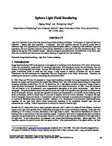
Fig. 3. Left: The light field consists of a predefined set of camera positions uniformly distributed on a sphere around the object. Middle: Only the opposing hemisphere is recorded for each camera. Right: The hemisphere is parameterised as parabolic environment map and stores both color and depth values.

of every camera for every pixel. Further pre-processing steps are necessary to generate the camera mesh and approximate a polygonal proxy representation of the object recorded or to extract per view depth maps for ray correction at rendering time. Rendering quality is closely related to the uniformity of the camera mesh and the complete covering of suitable viewing directions needed for reconstruction purposes. Due to the nature of the unstructured arrangement chosen for parametrisation, none of these two conditions can be guaranteed to be incorporated satisfactory. 3

S PHERICAL L IGHT F IELDS WITH P ER -P IXEL D EPTH

Our spherical light field rendering method with per-pixel depth correction of rays is inspired by ideas of Schirmacher et al. to use depth maps for ray correction [20] and profits from the uniformity of spherical parameterisations (see Section 2.2). Our approach directly works on combined RGB and depth image data to realize an efficient light field representation and high-quality light field rendering technique. In the remainder of this paper we refer to combined RGB and depth images short as RGBz images. The parameterisation is outlined in Figure 3. We employ a uniform spherical parameterisation to avoid discontinuity artefacts and guarantee full 6 DOF for virtual viewpoint selection. A virtual camera is located at each vertex of a regular, uniform triangulation of the sphere (left). For each camera an RGBz raster image of the opposing hemisphere is stored using a parabolic parameterisation (middle). The RGBz images for the individual cameras are stored on graphics hardware by writing the depth value in the alpha channel with every pixel (right). A standard color depth of 8 bit per RGBA channel is sufficient. This data representation is open for commodity texture compression algorithms. Light field reconstruction is performed by rendering the smooth shaded spherical proxy using a customized fragment program which performs effective per-pixel depth correction. 3.1

Spherical Camera Space Parameterisation

Our light field parameterisation is based on a spherical approximation to benefit from the uniformity of the sphere. A good polygonal approximation has to be generated for efficient storage and rendering. Platonic solids are known to be well suited for approximation of a sphere [5]. The most complex platonic solid is the icosahedron, a 20sided polyhedron with identical faces and vertex valences, providing an absolutely uniform distribution of vertices on the unit sphere. The icosahedron is thus a good choice as generator of uniform spherical approximations [4]. For further refinement we apply a recursive interpolatory subdivision scheme on the solid mesh (see Figure 4). With every iteration each triangle is divided into four (nearly) equilateral spherical triangles. As an optimization step we calculate the average length of all edges and iteratively adjust the vertex positions to obtain a most isometric tessellation.

Fig. 4. Spherical proxies are generated by successively subdividing the 20 faces of an icosahedron (left) into spherical approximations with 162 vertices (m = 2, middle) and 642 vertices (m = 3).

Applying the subdivision process m times, we obtain a spherical approximation with 20·4m faces. In practice, we chose m = 3 or m = 4, yielding 1280 or 5120 faces and 642 or 2562 vertices, respectively. The quality of a spherical approximation can be evaluated by means of the ratio of spherical surface area to approximated surface area. Ideally a tessellation into n patches should produce elements whose area is A = 4nπ . The icosahedron yields a surface area ratio of 76.08% of A, improving to 92.83% for m = 1, narrowing to 99.52% using m = 3 as shown in Figure 4. For a spherical light field representation m ≥ 3 is a good choice. The spherical approximation is stored explicitly as an indexed face set. With each vertex, a 4 × 4 viewing matrix is stored which represents the transformation of world to camera coordinates. This matrix is interpreted as extrinsic camera parameters for light field acquisition as well as for reconstruction purposes. 3.2 Parabolic Image Space Parameterisation For each camera, we store a 2D RGBz texture, which contains the recorded object projected onto the opposite hemisphere. Most viewing rays which hit the hemisphere centered around the camera will not hit the geometry. We thus avoid storing a second parabolic map for this hemisphere. As a consequence, the camera sphere √ must be larger than the object’s bounding sphere by a factor of 2 (see Figure 3, left). In Section 5 we will see that such a representation allows us to easily generate synthetic light fields from a highly tessellated geometry. Parabolic environment maps [9] provide the ideal solution for recording the hemisphere. They consume less storage than cube maps [8] and cause less distortion than both cube maps and spherical maps [16]. In practice, we chose a resolution of 256 × 256 or 512 × 512 pixels for each RGBz texture. The depth value is calculated as the distance z0 from the camera point to the object divided by the length of the ray secant zmax , according to Figure 5. This results in a depth value between 0 and 1, which can efficiently be stored as 8 bit alpha value. Storing the depth value as fractional part of the secant length also allows an efficient calculation of the object intersection point in the fragment program.

TECHNICAL REPORT, COMPUTER GRAPHICS GROUP, UNIVERSITY OF SIEGEN, 2007

4.1

The iterative refinement technique is outlined in Figure 6. When a triangle is rasterized, each fragment corresponds to a unique position Peye on the camera sphere. In the first step, the fragment program calculates the intersection point of the viewing ray with the camera (0) sphere to obtain a first estimate of the object intersection point Pobj . The superscript in this notation refers to the iteration count. The calculated intersection point is transformed into the viewing space of camera k according to

zmax

z'

Iterative refinement

(i)

Sk

Fig. 5. The depth value is obtained by dividing the camera-object distance z0 by the secant length zmax .

3.3 Texture Compression To reduce the amount of graphics memory consumed by the parabolic maps, commodity hardware-accelerated texture compression schemes can be employed. S3TC texture compression [11] offers an effective and easy way to compress the light field images. The DXT5 algorithm works on RGBA textures and achieves a compression ratio of 4:1. In our storage scheme, however, the alpha portion contains the depth values, which turn out to be sensitive to compression artefacts. To obtain best results for light field reconstruction we used the DXT3 algorithm. DXT3 works on RGBA data as well, but does not compress the alpha portion. DXT3 still offers a compression ratio of 4:1. A light field acquired using our spherical parameterisation with 642 images and a resolution of 512×512 pixels consumes 657 MB without compression. In comparison, a DXT3 compressed light field of the same dimensions consumes only 164 MB of memory. On commodity graphics cards, texture compression is thus mandatory to render light fields with 2562 cameras at interactive frame rates. Images 162 162 642 642 2562 2562

Resolution 256 × 256 512 × 512 256 × 256 512 × 512 256 × 256 512 × 512

Uncompressed 41.5 MB 165.9 MB 164.4 MB 657.5 MB 656.1 MB 2623.7 MB

S3TC DXT3 10.4 MB 41.5 MB 41.1 MB 164.4 MB 164.2 MB 656.1 MB

Table 1. Sizes of typical light fields with and without texture compression

4

L IGHT F IELD R ENDERING

The light field is rendered using a customized fragment program which requires a graphics processor that supports loop and conditional branch instructions according to shader model 3.0. We have implemented two different rendering techniques, both with per-pixel depth correction. The first one is an iterative refinement technique, which is more efficient in terms of runtime performance. The second one is a ray casting technique which is less efficient but more accurate. Both techniques will be outlined in the following. In both techniques the light field is rendered by rasterizing the front faces of the camera sphere with respect to the virtual viewpoint. The viewpoint is restricted to be located outside the camera sphere to avoid the vertices of the front faces being culled by frustum culling. Remember, each vertex corresponds to a pre-defined camera. For each triangle the parabolic RGBz texture images and the viewing matrices M of the three cameras are bound as uniform parameters to the fragment program. In practice the RGB and depth information of the parabolic map are bound as separate texture objects. While the RGB texture can be linearly interpolated, noticeable render artefacts at the silhouettes appear when interpolating the depth information. Using the nearest neighbour texture lookup scheme ensures appropriate depth information per pixel and avoids depth aliasing artefacts at object boundaries.

=

(i)

Mk Pobj

with

k ∈ {0, 1, 2}.

(2)

This is done for each of the three adjacent cameras that correspond to the original triangle’s vertices. The sphere intersection points Sk can now be converted to parabolic texture coordinates (u, v) , according to     µ ¶ s sx 1  1 +x sz + 1  u with Sk =  sy  . (3) = sy v k 2 +1 s 1 + sz

z

k

k

RGBz samples are obtained from the parabolic texture maps corresponding to the three cameras. The depth value z is extracted form the alpha portion and is used to calculate the camera’s local estimate (i) Pcam,k for the object intersection point: (i) (i) Pcam,k = z ·Ck + (1 − z) Pˆcam,k (i)

(4) (i)

with Pˆcam,k being the object intersection point Pobj projected onto the sphere using Ck as center of projection. Note that Equation 4 is a simple linear interpolation, because z stores the depth value as fractional part of the secant length (see Figure 5). An improved estimate for the object intersection point Pobj can now be found by projecting the three local camera distances onto the viewing ray and calculating the average, according to: (i+1)

Pobj

= Peye +

1 2 (i) ∑ ((Pcam,k −Ck ) · r) r 3 k=0

(5)

with r being the normalized direction of the original viewing ray (red line). As illustrated in Figure 6 (middle), the iteration can be pursued sev(i+1) eral times by projecting the updated object point Pobj onto the sphere using the camera vertices Ck as center of projection. The resulting intersection points are successively transformed into camera coordinates to establish depth values, to determine improved local estimates according to Equation 4 and eventually calculate an improved intersection point according to Equation 5. The procedure terminates if the desired accuracy is achieved or a maximum number of iterations is reached. In practice a maximum number of iterations of 5 turns out to be sufficient. The final color of the fragment is calculated as a weighted sum of the RGB values of the different cameras from the final iteration. The weights for each camera correspond to the barycentric coordinates of the fragment with respect to the original triangle. If the primary colors red, green and blue are assigned at the three vertices during geometry setup, the correct weights are automatically calculated through color interpolation during rasterization. Although this scheme allows the actual geometry intersection point to be approached quite quickly, unfortunately, the iterative refinement fails in certain situations. Such cases are illustrated in Figure 6, right. Case A shows a situation where the geometry is hit inside a concavity of the object, resulting in an intersection point that is not visible from at least one of the adjacent cameras. Case B illustrates a situation where the viewing ray does not hit the object at all, while at least one adjacent camera reports an intersection. These cases cannot be

SEVERIN TODT, CHRISTOF REZK-SALAMA AND ANDREAS KOLB: FAST (SPHERICAL) LIGHT FIELD RENDERING WITH PER-PIXEL DEPTH

A ^ (1) P cam,0 (0)

C0 Peye C1

Pcam,0

(0)

Pcam,1

(0) ^ (0) Pobj =P cam,k

C0

(1)

(1) Pcam,0 Pobj

C1

B

(1)

Pcam,1

^ (1) P cam,1

second iteration

first iteration

Fig. 6. Left and Middle: First and second step of the iterative depth refinement. Right: Iterative refinement fails at silhouette edges and locations where the correct object point is not visible from all adjacent cameras.

handled exactly and will inevitably result in visible ghosting artefacts at the silhouette edges. In order to extenuate such artefacts, we can examine the camera (i) estimates Pcam,k after a few iterations. If the three estimates are still highly divergent, we discard the point with the closest distance to the camera and proceed with the residual two cameras. If no similar local estimates can be achieved within the next few iterations, the averaging in Equation 5 is replaced by a maximum operation. This procedure, however, cannot completely eliminate the visual artefacts. If the ghosting is still too strong the only effective measure is increasing the number of cameras, or the image resolution. 4.2 Raycasting Approach The raycasting approach represents a less efficient, yet a simpler and more accurate solution to depth refinement. When a triangle is rasterized, the fragment program calculates the viewing ray, which corresponds to the fragment. We then calculate the intersection point of the viewing ray with the bounding sphere of the object.

C0

C1 C0

C1 C0

C1 Fig. 7. The raycasting approach samples the viewing ray stepwise at adjacent positions starting at the intersection point with the object’s bounding sphere.

From this position, we sample the viewing ray iteratively at a fixed step size, as shown in Figure 7. At each step, we validate the assumption that the current ray position is the actual object intersection point Pobj . We project this point onto the camera sphere using the adjacent camera positions Ck as center of projection. The resulting three intersection points with the sphere are transformed into the viewing coordinate system of the corresponding camera and converted to

parabolic coordinates. Depth values are obtained from the corresponding parabolic texture maps and local estimates Pcam,k are calculated for each camera according to Equation 4. We then compare these points to the position of the current ray sample. If one of the local estimates is equal to the ray position within a given tolerance, we immediately stop the ray sampling. This means that we have found at least one camera that reliably observes an object intersection at exactly the ray position. We now compare the intersection points obtained by the other two cameras. If they are also equal to the ray position within the given tolerance, we can assume that all cameras observe the same point and we use the barycentric weights of the fragment to calculate the final color for that pixel as outlined above. However, if the intersection point for one camera is far away from the ray position, we can assume that we are in one of the situations outlined in Figure 6 (right). In this case we discard the color information for the respective camera by setting the corresponding barycentric weight to zero. Afterwards, we normalize the weights again and calculate the final color as a weighted sum. 5

L IGHT F IELD G ENERATION

To obtain a light field from polygonal models, a virtual camera is applied at each spherical position determined by the camera space parameterisation. For synthetic light field acquisition based on 3D geometry, a given mesh is rendered once for each model camera. The viewing matrix is obtained from the spherical parameterisation. It transforms the scene such that the camera is placed at the position C = (0, 0, 1)T , looking along the negative z-axis. In this setup, the camera sphere is assumed to have unit radius. Hence, the entire scene has to be scaled and translated to fit into the bounding sphere with radius of √1 centered around the origin. 2 The vertex processor in the fixed-function graphics pipeline multiplies each vertex with the modelview and projection matrices before handing the primitives to the rasterization unit. The rasterizer assumes vertices to lie inside the canonical viewing volume which is equivalent to the unit cube [−1, 1]3 . For generation of synthetic light fields we replace this vertex processing step by a customized vertex program, which projects all vertices onto the unit sphere and converts the result to parabolic coordinates. This allows us to efficiently generate synthetic light fields using commodity graphics hardware. Due to the non-linear geometric distortions applied by our vertex program, however, it is mandatory to tessellate coarse geometry into small triangles before light field synthesis. On modern graphics hardware this can efficiently be achieved by a geometry shader program. The steps performed by our customized vertex program comprise the following. 1. Projection to the hemisphere. Each geometry vertex V is transformed with the modelview matrix and then projected from the camera point onto the opposite unit hemisphere. This is computed by casting a ray from the camera at position C = (0, 0, 1)T through the vertex and inter-

TECHNICAL REPORT, COMPUTER GRAPHICS GROUP, UNIVERSITY OF SIEGEN, 2007

secting this ray with the unit sphere. This amounts to solving a simple quadratic equation and results in a projected vertex S. 2. Parabolic mapping of the projected vertices As a result of the previous step, the projected vertex S is lying on the hemisphere with z < 0. The vertex S is converted to parabolic coordinates, according to Equation 3 3. Depth Adjustment The depth value is calculated according to Figure 5, which leads to kV −Ck (6) z= kS −Ck 4. Normal Transformation We assume that lighting is calculated in world coordinates. Hence, the normal vectors of the geometry must be transformed with the transposed inverse of the modeling matrix, but not with the viewing matrix. This, of course, is only necessary if the modeling matrix is not the identity matrix. As fragment shader to be used in combination with this customized vertex program, we can employ arbitrary complex fragment programs. The only modification necessary is that the fragment program must write the interpolated depth value generated by the vertex shader into the alpha portion of the final color. For each sample position RGB and depth values are stored in a parabolic map generated as described above. The alpha channel is used to store per-pixel depth information. Each parabolic map is stored as an interleaved array of RGBz values. Individual parabolic maps are associated with a transformation matrix defined by the spherical parameterisation. To store the set of parabolic maps additional header information is saved with the sample data for subsequent access and rendering of the light field. 6

R ESULTS AND D ISCUSSION

The techniques described in this paper have been implemented using OpenGL and Cg under Windows XP. All images and performance measurements have been created using an NVidia Geforce 8800 GTX graphics board with 768 MB of local video memory build into an AMD Athlon 64 X2 dual core processor with 2.21 GHz and 3.5 GB main memory. Figure 8 shows results of our light field rendering technique for camera spheres with different number of vertices. The light fields used to evaluate the system have been generated from highly tessellated polygonal geometry, as outlined in Section 5. The original polygonal geometry of the Stanford bunny is shown in the leftmost image in the upper row. During light field generation a surface shader with a high specular exponent was used to render the geometry resulting in sharp specular highlights. As has been shown in previous approaches [14, 7], specular highlights are critical to light field rendering, thus providing an excellent challenge to evaluate the accuracy of our implementation. All light fields in Figure 8 have an image resolution of 512 × 512. The remaining images in the top row show the tessellated camera sphere with 162, 642 and 2562 vertices, respectively. The second to fourth rows show images of the reconstructed light fields generated by our rendering techniques. Each row displays the results for a fixed resolution of the camera sphere. The two leftmost columns present example images created with our iterative refinement technique, the rightmost columns show the results of our raycasting technique. Each example image is supplemented by a difference image, which displays the pixel difference from the original geometry multiplied by a factor of 4 and inverted. These examples demonstrate the image quality obtained by our rendering technique. As expected, the iterative refinement technique produces noticeable ghosting artefacts at the silhouette edges, which are clearly visible in the difference images. The light fields with 162 vertices also show artefacts caused by the insufficient tessellation of the

sphere. The raycasting approach has significantly less ghosting artifacts at the silhouette edges. Note that for 642 and 2562 vertices, the difference images for raycasting approach only show reconstruction errors at the sharp specular highlights, which are strongly viewdependent. The bottom row of Figure 8 shows a light field with 2562 cameras reconstructed from the Lucy model. These images clearly demonstrate the advantages of the raycasting technique for complex geometries with fine details. The iterative refinement is not able to adequately capture the arm and the torch of the model, while the raycasting approach demonstrates that the depth information can be reconstructed accurately. This shows a clear weakness of the iterative refinement technique: Geometry intersection points which are closer to the camera than seen in any of the adjacent cameras cannot be determined with this technique. Table 2 shows the performance measured for rendering light fields of different resolution. The iterative refinement technique is much faster compared to the raycasting technique. This is not surprising, since the number of texture samples obtained for depth refinement is considerably smaller. The rendering process is clearly limited by the memory bandwidth between GPU and local video memory. Nevertheless, the results of our performance measurement show some aspects that are surprising. The first one is that the rendering speed is almost independent of the resolution of the texture images. The second surprising fact is that texture compression does not play a significant role to the runtime performance. This can be explained by the fact that our rendering techniques require only a very small and localized portion from each texture image, only a limited region seen by the respective camera. This small part of the texture fits easily into the texture cache. An exact comparison of performance and image quality to previously published solution to IBR is difficult to accomplish without access to the original implementations. To our knowledge the performance of our approach is at least equivalent to previous solutions reported in literature, even if we account for advances in hardware performance. The image quality achieved with our solution is significantly higher compared with previous solutions due to our perfragment depth refinement. The difference images prove that our solution is considerably close to the original. 7

C ONCLUSION

We have presented a novel GPU-based light field rendering technique based on combined RGB and depth information. We have demonstrated that this technique is capable of reconstructing light fields with high accuracy at interactive frame rates. For future development our aim is the possible acquisition of imagebased models using a hand-held camera with combined RGB and depth sensors. Recent progress in sensor technology have lead to the development of imaging devices which allow real-time measurement of per-pixel depth information [18, 24, 17, 6] at moderate resolution. In combination with RGB sensors these devices provide a promising alternative for accurate hand-held light field acquisition [18, 21]. With the direct usage of combined depth and RGB values as parabolic texture map, the presented approach is ready to be used for interactive light field acquisition with such a sensor setup. The next step towards the hand-held acquisition will be the implementation of a rebinning technique to successively insert recorded RGBz images into our light field representation. Since combined depth and RGB are evaluated directly by our rendering technique, immediate visual feedback will be available at acquisition time even for incomplete light field data. We are confident that the combination of spherical and parabolic parameterisation are ideal foundations to develop such a system in the near future. ACKNOWLEDGEMENTS We thank the members of the SFB-603 at the University of ErlangenNuremberg for their support. This research project is partially funded by grant KO-2960-6/1 from the German Research Foundation (DFG).

SEVERIN TODT, CHRISTOF REZK-SALAMA AND ANDREAS KOLB: FAST (SPHERICAL) LIGHT FIELD RENDERING WITH PER-PIXEL DEPTH

Images

Resolution

162 162 642 642 2562 2562

256 × 256 512 × 512 256 × 256 512 × 512 256 × 256 512 × 512

Uncompressed Raycasting 29.9 fps 29.9 fps 17.7 fps 17.2 fps 10.7 fps not applicable

Uncompressed Iterative Refinement 60.4 fps 60.3 fps 58.7 fps 58.3 fps 55.1 fps not applicable

S3TC DXT3 Raycasting 29.9 fps 29.9 fps 17.8 fps 17.6 fps 10.8 fps 10.4 fps

S3TC DXT3 Iterative Refinement 60.4 fps 61.7 fps 59.0 fps 58.8 fps 56.2 fps 56.1 fps

Table 2. Rendering performance for our raycasting rendering algorithm and the iterative refinement approach applied to light fields of varying resolution with and without texture compression.

R EFERENCES [1] E. H. Adelson and J. R. Bergen. The plenoptic function and the elements of early vision. In M. S. Landy and J. A. Movshon, editors, Computational Models of Visual Processing, pages 3–20. MIT Press, Cambridge, MA, 1991. [2] J. Blinn and M. Newell. Texture and reflection in computer generated images. ACM SIGGRAPH Comput. Graph., 10(2):266–266, 1976. [3] C. Buehler, M. Bosse, L. McMillan, S. Gortler, and M. Cohen. Unstructured lumigraph rendering. In Proc. ACM SIGGRAPH, pages 425–432, 2001. [4] E. Camahort, A. Lerios, and D. Fussell. Uniformly sampled light fields. Technical report, University of Texas at Austin, Austin, TX, USA, 1998. [5] P. Gasson. Geometry of Spatial Forms: Analysis, Synthesis, Concept Formulation and Space Vision for CAD. Ellis Horwood Series in Mathematics and its Applications. Ellis Horwood, Chichester, UK, 1983. [6] S. Gokturk, H. Yalcin, and C. Bamji. A time-of-flight depth sensor system description, issues and solutions. In Proc. IEEE Comp. Vis. and Pat. Rec. Workshop (CVPRW’04), page 35, 2004. [7] S. Gortler, R. Grzeszczuk, R. Szeliski, and M. Cohen. The lumigraph. In Proc. ACM SIGGRAPH, pages 43–54, 1996. [8] N. Greene. Environment mapping and other applications of world projections. IEEE Comput. Graph. Appl., 6(11):21–29, 1986. [9] W. Heidrich and H.-P. Seidel. Realistic, hardware-accelerated shading and lighting. In Proc. ACM SIGGRAPH, pages 171–178, 1999. [10] I. Ihm, S. Park, and R. Lee. Rendering of spherical light fields. In Proc. Pacific Graphics, page 59. IEEE Computer Society, 1997. [11] K. Iourcha, K. Nayak, and Z. Hong. System and method for fixed-rate block-based image compression with inferred pixel values. United States Patent 5,956,431, September 1999. S3 Incorporated (Santa Clara, CA). [12] S. Kang. A survey of image-based rendering techniques. In VideoMetrics, SPIE, volume 3641, pages 2–16. ACM Press, 1999. [13] J. Lengyel. The convergence of graphics and vision. Computer, 31(7):46– 53, 1998. [14] M. Levoy and P. Hanrahan. Light field rendering. In Proc. ACM SIGGRAPH, pages 31–42, 1996. [15] L. McMillan and G. Bishop. Head-tracked stereoscopic display using image warping. In Proc. ACM SIGGRAPH, pages 39–46, 1995. [16] G. Miller and C. Hoffman. Illumination and reflection maps: Simulated objects in simulated and real environments. In ACM SIGGRAPH Course Notes for Advanced Computer Graphics Animation, July 1984. [17] T. Oggier, B. B¨uttgen, F. Lustenberger, G. Becker, B. R¨uegg, and A. Hodac. SwissrangerT M SR3000 and first experiences based on miniaturized 3D-TOF cameras. In Proceedings, 1st Range Imaging Research Day, pages 97–108, ETH Zurich, Switzerland, September 2005. [18] T. Prasad, K. Hartmann, W. Wolfgang, S. Ghobadi, and A. Sluiter. First steps in enhancing 3D vision technique using 2D/3D sensors. In V. Chum, O.Franc, editor, Computer Vision Winter Workshop 2006, pages 82–86, University of Siegen, 2006. Czech Society for Cybernetics and Informatics. [19] H. Schirmacher, W. Heidrich, and H.-P. Seidel. High-quality interactive lumigraph rendering through warping. In Proc. Graphics Interface, pages 87–94, 2000. [20] H. Schirmacher, C. Vogelgsang, H.-P. Seidel, and G. Greiner. Efficient free form light field rendering. In VMV ’01: Proc. Vision Modeling and Visualization, pages 249–256. Aka GmbH, 2001. [21] S. S. Todt, C. Rezk-Salama, and A. Kolb. Real time fusion of range and light field images. In ACM SIGGRAPH 2005 Posters, page 65, 2005.

[22] C. Vogelgsang and G. Greiner. Hardware accelerated light field rendering. Technical Report 11, IMMD 9, Universitaet Erlangen-Nuernberg, 1999. [23] C. Vogelgsang and G. Greiner. Adaptive lumigraph rendering with depth maps. Technical Report 3, IMMD 9, Universitaet Erlangen-Nuernberg, 2000. [24] G. Yahav, G. J. Iddan, and D. Mandelboum. 3D imaging camera for gaming application. Technical Report, 3DV Systems Ltd., 2006.

TECHNICAL REPORT, COMPUTER GRAPHICS GROUP, UNIVERSITY OF SIEGEN, 2007

original geometry

162 cameras

642 cameras

Iterative Refinement

2562 cameras

Raycasting difference x4

difference x4

difference x4

difference x4

difference x4

2562 cameras

642 cameras

162 cameras

difference x4

original geometry

iterative refinement

raycasting

Fig. 8. Results of our light field rendering technique at different camera sphere resolutions. The first row shows the original geometry accompanied by polygonal spherical approximations of different resolutions used to generate synthetic views as shown in the following rows. Rows two to four display the rendering results for our iterative refinement rendering technique in comparison to the raycasting approach. Each synthetic view is supplemented by a difference image showing the pixel difference from the original geometry multiplied by a factor 4 and inverted. The bottom row presents a light field reconstruction of the Lucy model. It clearly shows the advantage of the raycasting technique for complex geometries with fine details.