Real-time Depth of Field Rendering via Dynamic Light Field ...

Volume 29 (2010), Number 7

Pacific Graphics 2010 P. Alliez, K. Bala, and K. Zhou (Guest Editors)

Real-time Depth of Field Rendering via Dynamic Light Field Generation and Filtering Xuan Yu 1 , Rui Wang 2 , and Jingyi Yu 1 1

Univ. of Delaware

2

Univ. of Massachusetts Amherst

Abstract We present a new algorithm for efficient rendering of high-quality depth-of-field (DoF) effects. We start with a single rasterized view (reference view) of the scene, and sample the light field by warping the reference view to nearby views. We implement the algorithm using NVIDIA’s CUDA to achieve parallel processing, and exploit the atomic operations to resolve visibility when multiple pixels warp to the same image location. We then directly synthesize DoF effects from the sampled light field. To reduce aliasing artifacts, we propose an image-space filtering technique that compensates for spatial undersampling using MIP mapping. The main advantages of our algorithm are its simplicity and generality. We demonstrate interactive rendering of DoF effects in several complex scenes. Compared to existing methods, ours does not require ray tracing and hence scales well with scene complexity. Categories and Subject Descriptors (according to ACM CCS): Generation—Display algorithms

1. Introduction Realistic depth-of-field (DoF) plays an important role in creating photographic effects in rendered images. With distribution ray tracing, DoF can be simulated by tracing many random rays sampled on the lens [CPC84], and integrating the radiance of each ray. Such a solution is accurate but takes a long time to compute. Accumulation buffer [HA90] reorganizes the rays as multiple pinhole cameras on the lens and then renders each individual camera using rasterization. Though fast, this technique requires repeated rendering of the scene, therefore provides only limited speed. Approximate solutions perform a spatially varying blur on a single view image [Rok93,LKC09,EH07], and the amount of blur is determined by the depth of each pixel. This approach is very fast but its accuracy is limited as the blurring can cross depth boundaries. Recent advances exploit parallel computation on the GPU to simulate high-quality DOF effects in real-time [KS07, KTB09, LES09, LES10]. The results are impressive, but they require decomposition of the geometry into discrete depth layers, which may lead to rendering artifacts, especially for complex scenes. In this paper, we present a new algorithm for efficient rendering of high-quality depth-of-field (DoF) effects. Our alc 2010 The Author(s)

c 2010 The Eurographics Association and Blackwell Publishing Ltd. Journal compilation Published by Blackwell Publishing, 9600 Garsington Road, Oxford OX4 2DQ, UK and 350 Main Street, Malden, MA 02148, USA.

I.3.3 [Computer Graphics]: Picture/Image

gorithm solves DoF rendering from the perspective of light field rendering. We start with a single rasterization of the scene, which we call the reference view. Instead of decomposing the depth into discrete layers, we aim to sample the light field of the scene by warping the reference view to nearby views. This is effectively a scatter-based approach that approximates how the scene looks like from a different but closeby view point. Our implementation uses NVIDIA’s CUDA to achieve parallel processing. We also exploit the GPU’s atomic operations to resolve visibility when multiple pixels warp to the same image location. We then directly synthesize DoF effects from the sampled light field. To reduce aliasing artifacts, we propose a novel image-space filtering technique that compensates for spatial undersampling using MIP mapping. The main advantages of our algorithm are its simplicity and generality. We demonstrate interactive rendering of DoF effects in several complex scenes. Compared to existing methods, ours does not require ray tracing and hence scales well with scene complexity. Figure 10 shows examples of our rendering computed at about 40 fps. 2. Previous Work. Depth-of-Field. The equations governing DoF are wellknown in literature work. Assume that a thin lens has focal

X. Yu & R. Wang & J. Yu / Real-time Depth of Field Rendering via Dynamic Light Field Generation and Filtering

Figure 2: A diagram showing the pipeline of our rendering algorithm. Figure 1: Thin lens model and lens light field. (a) The cause of defocus blurs. (b) Accumulation buffer reorganizes rays into cameras. (c) Our lens light field parameterization. length f , aperture size D (hence the f -number N = f /D), and the sensor is placed at 1 unit distance away from the lens. If the focal depth is s, applying the lens equation gives: 1 1 +1 = s f

(1)

For an arbitrary scene point p that is d(p) away from the lens, if p is closer than the focal depth (i.e., d(p) < s), p’s image will lie behind the image plane. This causes a circle of confusion with diameter b(p) as shown in Figure 1(a), where b(p) = α

| d(p) − s | d(s − β)

(2)

Here α = f 2 /N, and β = f . Similar defocus blurs occur for points that are fathers away than the focal depth. Post-Filtering Methods. Most real-time DoF methods rely on post-processing of a single pinhole image. Gatherbased methods [Rok93, Sch04, EH07, LKC09] apply a spatially varying blur at each pixel, and the amount of blur is determined by the circle of confusion size. This can be easily implemented on the GPU, leading to real-time performance. However, an image-space spatial blur often causes intensity leakage due to the fact that the blur can cross depth discontinuities [Dem04]. Scatter-based methods [PC81] map source pixels onto the circle of confusion and blend them from far to near. This requires depth sorting, which is costly even on modern GPUs. Our approach differs from these scatter-based methods in that we do not project directly to the circle of confusion; in addition, we exploit the GPU’s atomic operations to efficiently resolve depth visibility. While single-view methods are simple, they can lead to artifacts due to incorrect depth visibility. These artifacts can be effectively reduced using post-processing techniques

such as anisotropic diffusion [BFSC04, KB07, KLO06] or multi-layer fusion [LKC08,KTB09,KS07]. The recent work by Lee et al. [LKC09] combines a circular filter and anisotropic mipmapping to produce impressive DoF effects. Their method is sophisticated, but the goal of our work is to develop a simple yet effective technique to achieve similar rendering quality without using sophisticated filtering. Raytracing and Multiview Methods. Multi-view based techniques build upon the classical distributed ray tracing [CPC84]. The accumulation buffer technique [HA90] reorganizes the rays as if they originate from cameras sampled on the lens. It then renders each individual camera and accumulates the results. However, repeated rendering of the scene is expensive, therefore this technique is primarily used for offline applications. Two recent algorithms by Lee et al. [LES09, LES10] decompose the scene into depth layers and use image-based ray tracing techniques to rapidly compute DoF. Their method is able to achieve impressive results. However, the layer-based scene representation may lead to rendering artifacts, especially for complex scenes. Some recent work also studied DoF effects in micropolygon rendering, notably [FLB∗ 09] and [HQL∗ 10]. With a Reyes style rendering framework, these techniques can achieve production quality effects. But micropolygon rendering is currently still quite expensive, even by exploiting the GPU’s parallel processing power. Light Field Rendering. In this paper, we approach the problem of real-time DoF from the perspective of light field rendering. A light field [LH96] stores regularly sampled views looking at an object on a 2D sampling plane. These views form a 4D ray database and new views are synthesized by querying and blending existing rays. Given the light field of a scene, we can easily simulate DoF effects by integrating spatial and angular information in the light field. Isaksen et al. [IMG00] proposed to render DoF by reparameterizing the rays onto the focal plane and blending them via a wide aperture filter. Ng et al. [Ng05] proposed a similar technique in the Fourier space. Soler et al. [SSD∗ 09] applied Fourier c 2010 The Author(s)

c 2010 The Eurographics Association and Blackwell Publishing Ltd. Journal compilation

X. Yu & R. Wang & J. Yu / Real-time Depth of Field Rendering via Dynamic Light Field Generation and Filtering

Figure 3: (a) shows a synthesized light field view before hole filling. (b) shows the result after increasing the support size of each write. analysis in light transport to analyze adaptive sampling rate for DoF effects. Our method also builds on the wide aperture filter, but our focus is to develop real-time DoF algorithm by sampling the light field on the fly. 3. Dynamic Light Field Generation Figure 2 shows the pipeline of our algorithm. We start with rendering a reference view and its depth map using rasterization. We then generate a light field by warping the reference view onto an array of virtual light field cameras. Once we construct the light field, we then apply a wide aperture filter [IMG00] to synthesize DoF effects. Furthermore, we develop a simple but effective light field filtering technique to reduce aliasing artifacts caused by spatial undersampling. The core of our algorithm is to dynamically synthesize a light field from a single rasterized view. For the rest of the paper, we assume that our viewing camera has unit focal length (i.e., the sensor is at unit distance away from the lens), the vertical field-of-view (FoV) of the camera is θ, and the horizontal and vertical resolutions are w and h, respectively. 3.1. Lens Light Field Light fields provide an image-based representation that uses a set of rays to describe a scene in place of explicit geometry. A light field captures all the necessary rays within a certain sub-space so that every possible view within a region can be synthesized. In practice, a light field is stored as a 2D array of images. Each pixel in the image can be indexed as an integer 4-tuple (s,t, u, v), where (s,t) is the image index in the array and (u, v) is the pixel index in the image. Note that this camera-pixel representation differs from the classical two plane parametrization where (s,t, u, v) are defined under the world coordinate. In this paper, we construct a lens light field using the camera-pixel stuv parametrization. We assume that the st plane is the lens plane, and we put an array of virtual light field cameras on this plane. The light field cameras have c 2010 The Author(s)

c 2010 The Eurographics Association and Blackwell Publishing Ltd. Journal compilation

Figure 4: Light field warping. (a) Directly warping the color using the depth map leads to visibility problem. (b) We instead warp the depth values and apply the CUDA’s atomic min operation. identical parameters (FoV, resolution, focal depth, etc) as the viewing camera, and we use their pixel index as the uv coordinates of the ray. We further denote the sensor plane as the xy plane and the optical axis of the lens as the z direction. We use the central light field camera (i.e., (s,t) = (0, 0)) as the reference camera R00 and use Lout (s,t, u, v) to denote the lens light field. Our light field is similar to the in-camera light field in [Ng05]. The main difference is that we focus on modeling rays facing towards the scene whereas [Ng05] captures the in-camera rays back onto the xy plane. To distinguish between the two, we use Lin (x, y, s,t) to represent the incamera light field. A major advantage of using the camerapixel parametrization is that we can easily find all rays that pass through a 3D point P in terms of its disparity. Assume P is captured at pixel p(u0 , v0 ) on the reference camera and has depth z, we can compute the disparity of p using the following similarity relationship: disp =

h 1 · 2 tan(θ/2) z

(3)

For every light field camera Rst , we can find its pixel (ray) (u, v) that passes through P as: (u, v) = (u0 , v0 ) + disparity · (s,t)

(4)

We call Equation 4 the light field warping equation. In following section, we will use this equation to generate the light field. We will further apply the warping equation to synthesize DoF effects in Section 4. 3.2. Parallel Light Field Generation Our goal is to generate a light field from the reference view R00 . To do so, we first render the color and depth images at R00 using standard rasterization. We then warp the rendering result onto the rest of the light field cameras using Equation 4. We benefit from the NVIDIA CUDA architecture that allows parallel data scattering to achieve real-time performance. The DirectX compute shader can support similar functionality on DX 11 featured graphics cards.

X. Yu & R. Wang & J. Yu / Real-time Depth of Field Rendering via Dynamic Light Field Generation and Filtering

To generate the light field, a naive approach is to directly warp the RGB color of each pixel p(u0 , v0 ) in R00 onto other light field cameras. Specifically, using p’s depth value, we can directly compute its target pixel coordinate in camera Rst using the warping equation 4. Using parallel writes, we can simultaneously warp all pixels in R00 onto other light field cameras. This simple approach, however, results in incorrect visibility: multiple pixels in R00 that have different depth values may warp to the same pixel q in the light field camera Rst , as shown in Figure 4. To resolve the visibility problem, we choose to warp the disparity value instead of the pixel color, and we use the atomic min operation to resolve parallel write conflict. Our algorithm generates a disparity-map light field. To query the color of a ray (s,t, u, v), we can directly warp (u, v) back to (u0 , v0 ) in R00 using Equation 4. Although not the focus of this paper, the use of the depth light field has other advantages in efficient storage. For example, besides color and depth values, R00 can store other information such as surface normals and material properties. The depth light field allows one to quickly query these data without replicating them at each light field camera. Handling Holes. Although our warping algorithm is very efficient, it introduces holes in the resulting light field. There are two main causes for the holes. First, the disparity values that we use for warping are floating point numbers. Therefore, they introduces rounding errors when computing the target pixel coordinates. To fill in these holes, a naive approach is to super-sample the reference image. However, this requires higher computation cost. Instead, we adopt a simple scheme: when warping a pixel to its target position, we also write the pixel to its neighboring pixels, essentially increasing its support size. All write operations go through depth comparisons to ensure correct visibility. In our experiments, we find that this simple solution is quite effective at filling holes, as is shown in Fig.3. The second type of holes is caused by occlusion. Since our reference view does not contain information in occluded regions, we will not be able to accurately fill these holes. Although these holes can lead to severe artifacts in certain applications such as light field rendering, they are less problematic for rendering DoF. This is mainly because the size of the occlusion hole depends on the baseline between the light field cameras. If we fix the number of cameras in the lens light field, we incur more holes when using a wider aperture as the cameras will scatter more. On the other hand, wider apertures lead to shallower DoF – in other words, the out-offocus regions will appear blurrier. This implies that we can apply an image-space filtering technique to compensate for the missing holes. Refer to the discussion in the next section. 4. DoF Synthesis from the Light Field To synthesize DoF from the light field, we apply the wide aperture filter introduced in [IMG00].

4.1. In-Camera Light Field The image’s pixel values are proportional to the irradiance [SCCZ86] received at the sensor, computed as a weighted integral of the incoming radiance through the lens: I(x, y) ≈

ZZ

Lin (x, y, s,t) cos4 φds dt

(5)

where I(x, y) is the irradiance received at pixel (x, y), and φ is the angle between a ray Lin (x, y, s,t) and the sensor plane normal. This integral can be estimated as summations of the radiance along the sampled rays: I(x, y) ≈

∑ Lin (x, y, s,t) cos4 φ

(6)

(s,t)

Isaksen et al. [IMG00] directly applied Eqn. (6) to render the DoF effects. From every pixel p(x, y) on the sensor, one can first trace out a ray through lens center o to find its intersection Q with the focal plane. Then, Q is backprojected onto all light field cameras and blended with the corresponding pixels. Though simple, this approach requires back-projection that is not desirable for us. We avoid back-projection by reusing the warping equation. To do so, it is easy to verify that pixel p(x, y) in Rst to pixel (u0 , v0 ) = (w − x, h − y) in R00 , as shown in Figure 1. Therefore, if we assume the focal plane is at depth z0 , we can directly compute its corresponding focal disparity f disp using Eqn (3). Next, we can directly find the pixel index in camera Rst using Eqn. (4). The irradiance at p can then be estimated as: I(x, y) ≈

∑ Lout (s,t, u0 + s · f disp, v0 + t · f disp)

(7)

(s,t)

=

∑ Lout (s,t, w − x + s · f disp, h − y + t · f disp) (s,t)

To estimate the attenuation term cos4 φ, Isaksen et al. used a Gaussian function to approximate the weight on each ray. In contrast, we directly compute cos4 φ for each ray (s,t, u, v) without approximation. Specifically, the direction of each ray is (s,t, 1), thus cos4 φ = (s2 +t12 +1)2 . Finally we can query each ray using the depth light field described in Section 3 and blend them to synthesize the DoF effects. As explained in Section 3, our light field contains holes near occlusion boundaries. This implies that not every ray we query will have a valid value. Therefore, we mark the rays originating from the holes as invalid and discard them when computing irradiance at each pixel. 4.2. Anti-aliasing In order to reduce GPU texture memory consumption, we choose to render a small light field containing 36 to 48 cameras at a 512x512 image resolution. The small spatial resolution may lead to observable undersampling artifacts, which we solve by using jittered sampling and filtering. c 2010 The Author(s)

c 2010 The Eurographics Association and Blackwell Publishing Ltd. Journal compilation

X. Yu & R. Wang & J. Yu / Real-time Depth of Field Rendering via Dynamic Light Field Generation and Filtering

Figure 6: Comparing the rendering results with and without anti-aliasing. Figure 5: Synthesizing DoF using the focal plane. (a) Given a ray (yellow) from the reference camera, we find the rays (red) in the data cameras using the focal plane. (b) We then query and blend the rays to synthesize DoF. Sampling. We use jittered sampling of the light field to reduce aliasing. Specifically, we generate a Halton sequence and map it onto the lens light field as the camera positions [PH04]. The main advantage of using a Halton sequence is that it produces randomly distributed camera samples and is cheap to evaluate. Since our focal disparity model directly computes the pixel index for each light field camera Rst , incorporating jittered sampling does not require any additional change in our implementation. Filtering. We also develop a simple pre-filtering technique similar to the cone tracing method in [LES09]. Our method is based on the observation that an out-of-focus region exhibits the most severe aliasing artifacts as they blend rays corresponding to far away 3D points. This is demonstrated in Figure 6. On the other hand, out-of-focus regions generate significant blurs, thus accurately computing each ray is not necessary for these regions. This indicates that we can compensate for undersampling by first blurring the outof-focus rays and then blending them. A similar concept has been used in the Fourier slicing photography technique for generating a band-limited light field [Ng05]. To simulate low-pass filtering in light field rendering, we first generate a Mipmap from the reference image using a 3x3 Gaussian kernel. Gaussian Mipmaps eliminate the ringing artifacts and produce smoother filtering results than regular box-filters [LKC09]. We then directly use the Gaussian Mipmap in our light field ray querying process.

represents the spatial coverage of the ray cone in object h/2 space. tan(θ/2)·d is the pixel count per unit length which r transforms blur size (in object space) to the number of pixels (in image space). Figure 6 compares our rendering results with and without anti-aliasing. 5. Results and Analysis Our algorithm is tested on a PC with 2.13 Ghz Intel dual core CPU, 2GB meomry, and an NVIDIA Geforce GTX285 GPU. The light field generation and dynamic DoF rendering algorithms are implemented using NVIDIA CUDA 2.2 with compute capability 1.3. Rasterization of the reference views and anti-aliasing filtering are implemented using DirectX 9.0. All results are rendered by generating a dynamic light field with pixel resolution 512x512 and a default spatial resolution of 36. Note that with DirectX 11 and the compute shaders, it is possible to implement all algorithms without the resource mapping overheads between CUDA and DX. Performance: Table 1 summarizes the performance for each stage of the pipeline, as well as compares the performance under different spatial resolutions of the light fields. Instead of showing the overall fps, we use NVIDIA CUDA profiler to measure the exact running time that each CUDA kernel takes. Table 1 reveals that the rendering cost is dominated by the light field generation stage. In particular, the cost comes mainly from the atomic operation performed when warping the pixels (to account for correct visibility).

where dr is the depth value of pixel Pr , d f is the focal depth

Image Quality: In Figure 10, we compare the ground truth DoF results, the accumulation buffer results, and our results. The ground truth images are obtained using distributed ray tracing with 300 rays per pixel. We render equal number of views (36) for both the accumulation buffer and our approach. Both the ground truth and the accumulation buffer results are generated offline on the CPU. We observe that with the same number of views, accumulation buffer exhibits obvious aliasing artifacts whereas our approach produces nearly artifact-free results at interactive speed.

(c/N)·(dr −d f ) df

When the number of light field cameras is insufficient, our

Specifically, assume that the scene is focused at depth d f . When we query a ray (u, v) in camera Rst , we first obtain its depth value dr from the depth light field. Applying Equation 2, we can obtain the correct blur size. We then index it to the proper Mipmap level l, using   (c/N) · (dr − d f ) h/2 l = log2 · (8) df tan(θ/2) · dr of the camera, c is the diameter of the aperture.

c 2010 The Author(s)

c 2010 The Eurographics Association and Blackwell Publishing Ltd. Journal compilation

X. Yu & R. Wang & J. Yu / Real-time Depth of Field Rendering via Dynamic Light Field Generation and Filtering

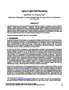
Figure 7: Illustrations of the four types of boundary artifacts. See Section 5 for details.

pixel of the virtual camera stores a disparity value of 4 bytes, a typical setting of 36 cameras with 512x512 resolution requires 36M GPU memory. We find this quite reasonable with the current generation of GPU. It is possible to keep only one virtual camera in video memory and accumulate each view one at a time, but that would split the computation and reduce parallelism, thus slowing down the performance. Boundary Artifacts: Next, we perform a detailed analysis on the boundary artifacts, and show how our light field based technique outperforms single-image filtering methods. We identify four canonical cases and examine them separately, although it is possible that a combination of these types of artifacts can simultaneously occur in rendering.

Figure 8: Comparing results generated by Image Space Blurring (a,c) and our light field synthesis (b,d). Our approach can efficiently reduce both the boundary discontinuities and intensity leakage artifacts. rendering results are subject to intensity leakage and boundary discontinuity artifacts. In the extreme case when only 1 light field camera is used, our method falls back to the naive image space blurring technique, as shown in Fig 9. Note the differences in the rendered results, especially near occlusion boundaries. In our experiments, we found that rendering a light field with 30 views is often sufficient to eliminate most visible boundary artifacts. Our Mipmap based image filtering is effective at reducing the undersampling artifacts when the spatial resolution of the light field is low. Memory Consumption. The memory consumption of our algorithm scales linearly with the number of virtual cameras, as well as each virtual camera’s image resolution. Since each

The first two cases occur when the camera is focused at the background. Consider a point Pb lying on the background whose image appears next to the foreground as shown in Figure 7(a). The ground truth result should properly blend both the foreground and background points. However, singleimage filtering techniques would consider Pb in focus and hence directly use its color as the pixel’s color. In this case, image-space blurring produces boundary discontinuity artifacts. In contrast, using our technique, rays originating from both the foreground and background will be captured by our synthesized light field, therefore our technique will produce the correct result. Next, we consider a point Pf on the foreground as shown in Figure 7(b). Similar to Pb , the ground truth result should blend a neighborhood of foreground points with a single background point (the focal point). Single-image filtering methods will assign a large blur kernel to Pf and hence blend a group of points on both the foreground and the background. This leads to incorrect results, except if the background points all have similar color. Our method, in contrast, will attempt to blend rays from both the foreground and the background. However, due to occlusion, background points are labeled missing, marked as dashed lines in Figure 7(b). c 2010 The Author(s)

c 2010 The Eurographics Association and Blackwell Publishing Ltd. Journal compilation

X. Yu & R. Wang & J. Yu / Real-time Depth of Field Rendering via Dynamic Light Field Generation and Filtering

Views 12 24 36 48 64

Wrapping (µs) 4996 9477 14238 19191 25111

Synthesis (µs) 1974 3850 5731 7592 10117

Total (s) 0.00697 0.013327 0.019969 0.026783 0.035228

Table 1: Performance profiles of CUDA kernels for the light filed generation step and DoF Synthesis step. We render the bunny scene with a wide aperture at a 512x512 image resolution, and vary the spatial revolution of the light field. In this case our method will discard these rays in the blending process, and hence also produces incorrect results manifested by boundary discontinuities. Analogous to the first two cases, the other two cases occur when the camera is focused at the foreground. Consider again a point Pb lying on the background, as shown in Figure 7(c). The ground truth result should blend points on the background, while the single-image filtering techniques will blend both the foreground and background points, leading to incorrect results. Our method attempts to blend rays originating from the background. However, due to occlusion, it can only access a portion of them. Therefore, if the background has similar color, it would produce reasonable results. Finally, consider again a point Pf on the foreground as shown in Figure 7(d). The ground truth will collect all rays from Pf and since these rays are all accessible to our light field, our method is also able to obtain the correct result. The single-image blurring method will produce correct result as well, since it will identify the pixel as in-focus and hence directly use Pf ’s color. Our analysis illustrates that, of the four cases, our approach correctly handles two (Figure 7(a,d)), reasonably approximates one (Figure 7(c)), and incorrectly handles one (Figure 7(b)). In contrast, single-image filtering techniques only handles one case correctly, one case reasonably well (Figure 7(d)), and the remaining two cases incorrectly. Figure 8 compares the rendering results using our method and the single-image filtering approach on an elephant scene. Our technique exhibits fewer visual artifacts compared to the single-image filtering method. In fact, our technique will not cause intensity leakage under any circumstance. 6. Conclusions and Future Work We have presented an efficient framework for realtime simulation of high-quality depth-of-field (DoF) effects. Our method approaches the DoF problem from the perspective of light field rendering. Our technique combines the benefits of both multi-view accumulation buffer and single-view filtering: by synthesizing and then rendering from a light field, we resolve the visibility problem in most cases; and by applying image-space filtering, we are able to effectively reduce the aliasing artifacts. Our algorithm is also easy to implement: c 2010 The Author(s)

c 2010 The Eurographics Association and Blackwell Publishing Ltd. Journal compilation

it directly uses the disparity warping model, and it builds upon the CUDA framework for general purpose GPU programming. By synthesizing as few as 36 light field views, our technique is able to produce DoF effects with quality comparable to raytraced reference. The main limitation of our technique is that it cannot synthesize light field rays near occlusion boundaries. As a result, our method can lead to boundary artifacts when the camera focuses at the background, as is shown in Section 5. The simplest solution is to apply GPU ray tracing for filling the holes. However, tracing missing rays in a large number of views may be challenging for interactive rendering. An alternative is to integrate our technique with the recently proposed occlusion camera model [PA06]. An occlusion camera uses non-pinhole geometry to "see-behind" the occlusions. Therefore, if we use the occlusion camera as our reference light field camera, we may be able to fill in many missing rays to further improve our rendering quality. We also plan to investigate the use of synthesized light field to render other challenging effects such as motion blur and glossy reflections. The recently proposed imagespace gathering [RS09] technique shares similar concepts with ours and has shown promising results. However, their method requires a parameter (ray) search stage while we directly lookup using the light field. In the future, we will investigate possible combinations of the two techniques for rendering a broader class of rendering effects. Acknowledgments We would like to thank the PG anonymous reviewers for their valuable comments and suggestions. The Fairy and toasters models are courtesy of Ingo Wald. Xuan Yu and Jingyi Yu are supported in part by NSF grants MSPAMCS-0625931 and IIS-CAREER-0845268; Rui Wang is supported in part by NSF grant CCF-0746577. References [BFSC04] B ERTALMIO M., F ORT P., S ANCHEZ -C RESPO D.: Real-time, accurate depth of field using anisotropic diffusion and programmable graphics cards. In Proc. of 3DPVT ’04 (2004), pp. 767–773. 2 [CPC84] C OOK R. L., P ORTER T., C ARPENTER L.: Distributed ray tracing. Proc. of SIGGRAPH ’84 18, 3 (1984), 137–145. 1, 2 [Dem04] D EMERS J.: Depth of field: A survey of techniques. GPU Gems 23 (2004), 375–390. 2 [EH07] E ARL H AMMON J.: Practical post-process depth of field. GPU Gems 3 28 (2007), 583–606. 1, 2 [FLB∗ 09] FATAHALIAN K., L UONG E., B OULOS S., A KELEY K., M ARK W. R., H ANRAHAN P.: Data-parallel rasterization of micropolygons with defocus and motion blur. In Proc. of HPG ’09 (2009), pp. 59–68. 2 [HA90] H AEBERLI P., A KELEY K.: The accumulation buffer: hardware support for high-quality rendering. In Proc. of SIGGRAPH ’90 (1990), pp. 309–318. 1, 2 [HQL∗ 10] H OU Q., Q IN H., L I W., G UO B., Z HOU K.: Micropolygon ray tracing with defocus and motion blur. ACM Trans. Graph. 29, 3 (2010), to appear. 2

X. Yu & R. Wang & J. Yu / Real-time Depth of Field Rendering via Dynamic Light Field Generation and Filtering

Figure 9: Comparing our results using a different number of light field cameras. [IMG00] I SAKSEN A., M C M ILLAN L., G ORTLER S. J.: Dynamically reparameterized light fields. In Proc. of SIGGRAPH ’00 (2000), pp. 297–306. 2, 3, 4

[Rok93] ROKITA P.: Fast generation of depth of field effects in computer graphics. Computers & Graphics 17, 5 (1993), 593– 595. 1, 2

[KB07] KOSLOFF T. J., BARSKY B. A.: An Algorithm for Rendering Generalized Depth of Field Effects Based on Simulated Heat Diffusion. Tech. Rep. UCB/EECS-2007-19, UC Berkeley, 2007. 2

[RS09] ROBISON A., S HIRLEY P.: Image space gathering. In Proc. of HPG ’09 (2009), pp. 91–98. 7

[KLO06] K ASS M., L EFOHN A., OWENS J.: Interactive depth of field using simulated diffusion on a GPU. Tech. rep., UC Davis, 2006. 2

[Sch04] S CHEUERMANN T.: Advanced depth of field. GDC (2004). 2

[KS07] K RAUS M., S TRENGERT M.: Depth-of-field rendering by pyramidal image processing. In Proc. of Eurographics 2007 (2007). 1, 2

[SCCZ86] S TROEBEL L., C OMPTON J., C URRENT I., Z AKIA R.: Photographic Materials and Processes. Focal Press, 1986. 4

[SSD∗ 09] S OLER C., S UBR K., D URAND F., H OLZSCHUCH N., S ILLION F.: Fourier depth of field. ACM Trans. Graph. 28, 2 (2009), 1–12. 2

[KTB09] KOSLOFF T. J., TAO M. W., BARSKY B. A.: Depth of field postprocessing for layered scenes using constant-time rectangle spreading. In Proc. of Graphics Interface ’09 (2009), pp. 39–46. 1, 2 [LES09] L EE S., E ISEMANN E., S EIDEL H.-P.: Depth-of-field rendering with multiview synthesis. ACM Trans. Graph. 28, 5 (2009), 1–6. 1, 2, 5 [LES10] L EE S., E ISEMANN E., S EIDEL H.-P.: Real-time lens blur effects and focus control. ACM Trans. Graph. 29, 3 (2010), to appear. 1, 2 [LH96] L EVOY M., H ANRAHAN P.: Light field rendering. In Proc. of SIGGRAPH ’96 (1996), pp. 31–42. 2 [LKC08] L EE S., K IM G. J., C HOI S.: Real-Time Depth-ofField Rendering Using Splatting on Per-Pixel Layers. Computer Graphics Forum (Proc. Pacific Graphics’08) 27, 7 (2008), 1955– 1962. 2 [LKC09] L EE S., K IM G. J., C HOI S.: Real-time depth-offield rendering using anisotropically filtered mipmap interpolation. IEEE Transactions on Visualization and Computer Graphics 15, 3 (2009), 453–464. 1, 2, 5 [Ng05] N G R.: Fourier slice photography. ACM Trans. Graph. 24, 3 (2005), 735–744. 2, 3, 5 [PA06] P OPESCU V., A LIAGA D.: The depth discontinuity occlusion camera. In Proc. of I3D ’06 (2006), pp. 139–143. 7 [PC81] P OTMESIL M., C HAKRAVARTY I.: A lens and aperture camera model for synthetic image generation. In Proc. of SIGGRAPH ’81 (1981), pp. 297–305. 2 [PH04] P HARR M., H UMPHREYS G.: Physically Based Rendering: From Theory to Implementation. Morgan Kaufmann Publishers Inc., San Francisco, CA, USA, 2004. 5 c 2010 The Author(s)

c 2010 The Eurographics Association and Blackwell Publishing Ltd. Journal compilation

X. Yu & R. Wang & J. Yu / Real-time Depth of Field Rendering via Dynamic Light Field Generation and Filtering

Figure 10: Comparing results generated with (a) distributed ray tracing (reference), (b) accumulation buffer with 36 views, and (c) our dynamic light field synthesis with 36 views. Our algorithm produces nearly artifact-free renderings in all three examples.

c 2010 The Author(s)

c 2010 The Eurographics Association and Blackwell Publishing Ltd. Journal compilation