Using a Simulated Annealing Algorithm to Solve the ... - CiteSeerX

Using a Simulated Annealing Algorithm to Solve the Transit Route Network Design Problem Wei Fan1 and Randy B. Machemehl2 Abstract: This paper uses a simulated annealing algorithm to solve the optimal bus transit route network design problem 共BTRNDP兲 at the distribution node level. A multiobjective nonlinear mixed integer model is formulated for the BTRNDP. The proposed solution framework consists of three main components: An initial candidate route set generation procedure that generates all feasible routes incorporating practical bus transit industry guidelines; and a network analysis procedure that assigns transit trips, determines service frequencies, and computes performance measures; and a simulated annealing procedure that combines these two parts, guides the candidate solution generation process and selects an optimal set of routes from the huge solution space. Three experimental networks are successfully tested as a pilot study. A genetic algorithm is also used as a benchmark to measure the quality of the simulated annealing algorithm. The presented numerical results clearly indicate that the simulated annealing outperforms the genetic algorithm in most cases using the example networks. Sensitivity analyses are performed and related characteristics and tradeoffs underlying the BTRNDP are also discussed. DOI: 10.1061/共ASCE兲0733-947X共2006兲132:2共122兲 CE Database subject headings: Routes; Network design; Algorithms; Travel demand; Simulation; Transportation management.

Introduction Public transit has been widely recognized as a potential way of reducing air pollution, lowering energy consumption, improving mobility, and lessening traffic congestion. Designing an operationally and economically efficient bus transit network is very important for the urban areas’ social, economic, and physical structure. Basically, the network design problem involves the minimization 共or maximization兲 of some intended objective subject to a variety of constraints, which reflect system performance requirements and/or resource limitations. In the past decade, several research efforts have examined the bus transit route network design problem 共BTRNDP兲. Previous approaches that were used to solve the BTRNDP can be classified into three categories: 共1兲 Practical guidelines and ad hoc procedures; 共2兲 analytical optimization models for idealized situations; and 共3兲 metaheuristic approaches for more practical problems. National Cooperative Highway Research Program 共NCHRP兲 Synthesis of Highway Practice 69 共1980兲 provides industry rules-of-thumb service planning guidelines. Furthermore, in the early stages of the research on BTRNDPs traditional operations research 1 Senior Optimization Developer, SAS Institute Inc., 100 SAS Campus Dr., Building R, Cary, NC 27513 共corresponding author兲. E-mail: [email protected] 2 Professor and Director, Center for Transportation Research, Dept. of Civil Engineering, The Univ. of Texas at Austin, 1 University Station, C1761, ECJ 6.908, Austin, TX 78712. E-mail: [email protected] Note. Discussion open until July 1, 2006. Separate discussions must be submitted for individual papers. To extend the closing date by one month, a written request must be filed with the ASCE Managing Editor. The manuscript for this paper was submitted for review and possible publication on February 8, 2005; approved on July 5, 2005. This paper is part of the Journal of Transportation Engineering, Vol. 132, No. 2, February 1, 2006. ©ASCE, ISSN 0733-947X/2006/2-122–132/$25.00.

analytical optimization models were used. Rather than determine both the route structure and design parameters simultaneously, these analytical optimization models were primarily applied to determine one or several design parameters 共e.g., stop spacing, route spacing, route length, bus size, and/or frequency of service兲 on a predetermined transit route network structure. Examples of these models can be seen in the work of Newell 共1979兲 and Leblanc 共1988兲. Basically, these analytical optimization models are very effective in solving optimization-related problems for networks of small size or with one or two decision variables. However, when it comes to the transit route design problem for a network of realistic size in which many parameters need to be determined, this approach does not work very well. Due to the inherent complexity involved in the BTRNDP, the meta-heuristic approaches, which pursue reasonably good local optima but do not guarantee to find the global optimal solution, were therefore proposed. The meta-heuristic approaches primarily dealt with simultaneous design of the transit route network and determination of its associated bus frequencies. Examples of the general heuristic approaches can be seen in the work of Lampkin and Saalmans 共1967兲, Rea 共1971兲, Silman et al. 共1974兲, Dubois et al. 共1979兲, Ceder and Wilson 共1986兲, and Ceder and Israeli 共1998兲. Artificial intelligence-based methods are used in Hasselstrom 共1981兲, Van Nes et al. 共1988兲, Baaj and Mahmassani 共1991兲, and Shih et al. 共1998a,b兲. Literature using genetic algorithm-based approaches to solve the BTRNDP can be seen in Pattnaik et al. 共1998兲, Chien et al. 共2001兲, and Fan and Machemehl 共2004兲. Previous heuristic solution methods use either artificial intelligence or genetic algorithms. However, other candidate heuristic methods, such as simulated annealing, have received much less attention. Furthermore, to make the BTRNDP tractable, several assumptions were made and the problems were oversimplified, making their solutions questionable and therefore preclude them as generally accepted applications for practical transportation networks. One example is that when the BTRNDP is studied

122 / JOURNAL OF TRANSPORTATION ENGINEERING © ASCE / FEBRUARY 2006

Downloaded 25 Jul 2011 to 146.6.92.226. Redistribution subject to ASCE license or copyright. Visit http://www.ascelibrary.org

in the context of the “distribution node” level 共i.e., without aggregating zonal travel demand into a single node兲, the frequency-based rule for the traditional transit trip assignment model is incorrect. Another example is that these models did not consider the phenomenon of the long-walk paths where transit users might walk a tolerable distance to their neighboring zones to take the bus. This situation might commonly exist when there is no direct service provided for transit users at a specific zone but provide such service at their neighbors. Therefore, the BTRNDP should be considered in a more general real world situation. In addition, there is a difference in needs that some transit agencies want to develop a new transit network from scratch while others intend to redesign their current transit networks so that they can be more efficient. In addition to the new design of transit networks as previous approaches studied, a more generalized solution methodology should be able to handle the redesign of the transit networks as well. This objective of this paper is to systematically examine the underlying characteristics of the optimal bus transit route network design problem in the context of the distribution node level. A multiobjective nonlinear mixed integer model is developed. A general simulated annealing-based solution methodology is proposed and numerical results including sensitivity analyses are presented for an experimental network. The subsequent sections of this paper are organized as follows. We first present model formulation of the BTRNDP from a systematic view. The objective function and related constraints are also described. Then, we propose the solution methodology for the BTRNDP, which contains three main components: An initial candidate route set generation procedure 共ICRSGP兲; a network analysis procedure 共NAP兲, and a simulated annealing 共SA兲 algorithm-based meta-heuristic implementation model that combines the first two parts. Next, we present the applications of the proposed solution methodology to an experimental network and the numerical results are also discussed. Finally, we conclude this paper with a summary.

Model Formulation In essence, the transportation system can be described in terms of “nodes,” “links,” and “routes.” A node is used to represent a specific point for loading, unloading and/or transfer in a transportation network. Basically, there are three kinds of nodes in a bus transit network system: 共1兲 Nodes representing centroids of specific zones; 共2兲 nodes representing road intersections; and 共3兲 nodes with which zone centroid nodes are connected to the network through centroid connectors. Note that nodes could be real identifiable on the ground or fictitious. Furthermore, the term distribution nodes is introduced especially for the third kind of nodes. A link joins a pair of nodes and represents a particular mode of transportation between these nodes, which means that if different modes of transportation are involved with the same link, these are represented as two links, say walk mode and transit mode. This is natural since the travel time associated with every mode specific link is different. A route is a sequence of nodes. Every consecutive pair of the node sequence must be connected by a link of the relevant mode. The bus line headway on any particular route is the interarrival time of buses running on that route. A graph 共network兲 refers to an entity G = 兵N , A其 consisting of a finite set of N nodes and a finite set of A links 共arcs兲 which connect pairs of nodes. A transfer path is a progressive path that uses more than one route. Note that a typical geographical zone

system may be based upon census boundaries and all land areas are encompassed by streets or major physical barriers. The zone centroids are located somewhere near the centers of the zones and zone connectors are used to connect these centroids to the modeled network. Generally, the centroid node represents the “demand” center 共origin and/or destination兲 of a specific traffic zone. Distribution nodes are the junctions of centroid connectors and road links. It should be pointed out that centroid connectors are usually fictitious and they are used as the origins and/or destinations for implementation of the shortest path and k-shortest path algorithms. Furthermore, an important characteristic of these centroid connectors is the distances that transit users have to walk to get to the routes that provide service to their intended destinations. Note that the terms, “arc” and link are used interchangeably. Consider a connected network composed of a directed graph G = 兵N , A其 with a finite number of nodes, N connected by A arcs. The following notations are used. Sets/Indices i , j 苸 N⫽centroid nodes 共i.e., zones兲; rk 苸 R⫽routes; it 苸 N⫽tth distribution node of centroid node i; and tr 傺 R⫽transfer paths that use more than one route from R. Data Rmax⫽maximum allowed number of routes for the route network; Umax⫽percentage of maximum allowed unsatisfied transit demand; N⫽number of centroid nodes in the route network; Dmax⫽maximum length of any route in the transit network; Dmin⫽minimum length of any route in the transit network; dij⫽bus transit travel demand between centroid nodes i and j; hmax⫽maximum headway required for any route; hmin⫽minimum headway required for any route; Lmax⫽maximum load factor for any route; P⫽seating capacity of buses operating on the network; W⫽maximum bus fleet size available for operations on the route network; Cv⫽per-hour operating cost of a bus 共$/vehicle/h兲; Cm⫽value of time 共$/min兲; Ov⫽operating hours for the bus running on any route 共h兲; Cd⫽value of one unsatisfied transit demand in dollars 共$/person兲; and C1 , C2 , C3⫽weights reflecting the relative importance of three components including the user costs, operator costs and unsatisfied total demand costs, respectively, note that C1 + C2 + C3 = 1. Decision Variables M⫽number of routes of the current proposed bus transit network solution; rm⫽mth route of the proposed solution, m = 1 , 2 , . . . , M; Drm⫽overall length of route rm; drijm⫽bus transit travel demand between centroid nodes i and j on route rm; dtrij ⫽bus transit travel demand between centroid nodes i and j along transfer path tr; DRij⫽set of direct routes used to serve the demand from centroid nodes i and j; TRij⫽set of transfer paths used to serve the demand from centroid nodes i and j; trijm⫽total travel time between centroid node i and j on route rm; ttrij ⫽total travel time between centroid node i and j along transfer path tr; hrm⫽bus headway operating on route rm共min/ vehicle兲; Lrm⫽loading factor in route rm; Trm⫽round trip time of route rm; Nrm⫽number of operating buses required on route rm; Nrm = Trm / hrm; and Qrmax⫽maximum m flow occurring on the route rm.

JOURNAL OF TRANSPORTATION ENGINEERING © ASCE / FEBRUARY 2006 / 123

Downloaded 25 Jul 2011 to 146.6.92.226. Redistribution subject to ASCE license or copyright. Visit http://www.ascelibrary.org

Objective Function The objective is to minimize the sum of user cost, operator cost, and unsatisfied demand costs for the studied bus transit network. The objective function is as follows: min z = C1 ·

冉兺 兺

兺

i苸N j苸N rm苸DRij

Cv · Ov · + C2 · Cm ⫻

冉兺 兺

dij −

i苸N j苸N

drijmtrijm +

冉兺 冊 M

m=1

T rm h rm

兺兺 兺

dtrij ttrij

i苸N j苸N tr苸TRij

+ C3 ·

兺兺 兺

i苸N j苸N rm苸DRij

冊

Cd Cm

drijm −

兺兺 兺

dtrij

i苸N j苸N tr苸TRij

冊

such that hmin 艋 hrm 艋 hmax

rm 苸 R

constraint represents the resource limits of the transit company and it guarantees that the optimal network pattern never uses more vehicles than the currently available ones. The fourth constraint is the trip length constraint. This avoids routes that are too long because bus schedules on very long routes are too difficult to maintain. Meanwhile, to guarantee the efficiency of the network, the length of routes should not be too small. The fifth constraint is the maximum number of routes constraint, which reflects the fact that in solving the BTRNDP, transit planners often set a maximum number of routes, which is based on the fleet size, and this will have a great impact on the later driver scheduling work. The sixth constraint specifies that the maximum allowed unsatisfied demand cannot exceed a specific user-defined percentage of the total transit demand.

共headway feasibility constraint兲

Proposed Solution Methodology L rm =

· h rm Qrmax m P

M

M

艋 Lmax

T rm

兺 Nr = m=1 兺 hr m=1 m

艋W

共fleet size constraint兲

rm 苸 R

共trip length constraint兲

共maximum numbers of routes constraint兲

兺兺 兺 i苸N j苸N r 苸DR m

rm 苸 R

共load factor constraint兲

m

Dmin 艋 Drm 艋 Dmax M 艋 Rmax

rm 苸 R

drijm + ij

艌 共1 − Umax兲 ·

兺兺 兺 i苸N j苸N tr苸TR

dtrij

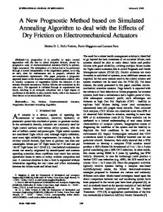
The proposed solution framework consists of three main components: an ICRSGP that generates all feasible routes incorporating practical guidelines that are commonly used in the bus transit industry; a NAP that assigns the transit trips, determines the service frequencies on each route, and computes many performance measures, and a SA procedure that combines these two parts, guides the candidate solution generation process, and selects an optimal set of routes from the huge solution space. Fig. 1 gives the flow chart of the proposed solution framework. In addition, C + + is chosen as the implementation language in this paper. Details of the proposed solution methodology are presented as follows.

ij

兺 兺 dij

ICRSGP

i苸N j苸N

共maximum allowed unsatisfied transit demand constraint兲 where M, hrm, Nrm, Qrmax, drijm, and dtrij ⫽integers. m The first term of the objective function is the total user cost 共including the user cost on direct routes and that on transfer paths兲, the second part is the total operator cost, and the third component is the cost resulting from total transit demand excluding those satisfied by a specific network configuration. Note that C1, C2, and C3 are introduced to reflect the tradeoffs between the user costs, the operator costs and unsatisfied transit ridership, making BTRNDP a multiobjective optimization problem. Generally, operator cost refers to the cost of operating the required buses. User costs usually consist of four components, including walking cost, waiting cost, transfer cost, and in-vehicle travel cost. However, to the authors’ knowledge, almost all of the previous research on the BTRNDP did not include the cost of unsatisfied demand. This point is quite obvious because the optimal solution to the BTRNDP without considering unsatisfied demand costs should be “no service provided at all” and the “zero” cost could always be the best solution that one can achieve for the minimization problem. Therefore, inclusion of unsatisfied demand cost in the objective function is justified. The first constraint is the headway feasibility constraint, which reflects the necessary usage of policy headways on extreme situations. The second is the load factor constraint, which guarantees that the maximum flow on the critical link of any route rm cannot exceed the bus capacity on that route. The third 共fleet size兲

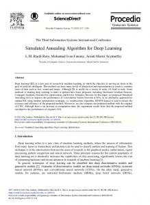
The ICRSGP configures all candidate routes for the current transportation network. It requires the user to define the minimum and maximum route lengths. The knowledge of the transit planners has a significant impact on the initial route set skeletons, that is, different user requirements may result in different route solution space sets. ICRSGP relies mainly on algorithmic procedures including the shortest path and k-shortest path algorithms. Given the user-defined minimum and maximum length constraints, Dijkstra’s shortest path algorithm 共Ahuja et al. 1993兲 is used and Yen’s k-shortest path algorithm 共Yen 1971兲 is modified to generate all candidate feasible routes in the studied transportation network. Fig. 2 presents a flow chart for the ICRSGP. In Step 1, ICRSGP starts by using Dijkstra’s label-setting shortest path algorithm to find the shortest path P共i , j兲 between each centroid node pair 共i , j兲 in the bus transit demand network. Each of these paths may form a feasible route element in the optimal bus transit route network solution space. In Step 2, the initial set of all routes generated in Step 1 is checked by two feasibility filter tests: 共1兲 Minimum route length constraints; and 共2兲 maximum route length constraints. Routes that pass these two tests will be kept. The distance of these respective routes will be recorded and a label will be set to keep track of each one. In Step 3, all alternate routes are generated using modified Yen’s kth shortest path algorithm between the same origin and destination as that generated in Step 1. At each step, the generated path is checked for Step 4 until all feasible routes have been generated In Step 4, the initial

124 / JOURNAL OF TRANSPORTATION ENGINEERING © ASCE / FEBRUARY 2006

Downloaded 25 Jul 2011 to 146.6.92.226. Redistribution subject to ASCE license or copyright. Visit http://www.ascelibrary.org

Fig. 1. Flow chart of the proposed solution methodology

candidate route set generation algorithm checks the route fundamental feasibility for each present route generated in Step 3. All feasible routes that satisfy these constraints are kept and labeled, and all the leftovers are removed. In Step 5, the ICRSGP stores all the routes with their respective labels as elements of the overall candidate solution route set.

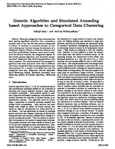
NAP Fig. 3 shows the flow chart of the proposed network analysis procedure for the BTRNDP. As can be seen, the NAP proposed in this paper is a bus transit network evaluation tool with the ability to assign the transit trips between each centroid node pair to each

Fig. 2. Skeleton of the ICRSGP JOURNAL OF TRANSPORTATION ENGINEERING © ASCE / FEBRUARY 2006 / 125

Downloaded 25 Jul 2011 to 146.6.92.226. Redistribution subject to ASCE license or copyright. Visit http://www.ascelibrary.org

Fig. 3. NAP for the BTRNDP

route on the proposed solution network and determine associated route frequencies. To accomplish these tasks for the BTRNDP, NAP employs an iterative procedure, which contains two major components, namely, a multiple transit trip assignment procedure and a frequency setting procedure, to seek to achieve internal consistency of the route frequencies. Once a specific set of routes is proposed in the overall candidate solution route set generated by the ICRSGP, the NAP is called to evaluate the alternative network structure and determine

route frequencies. The whole NAP process can be described as follows. First, an initial set of route frequencies are specified because they are necessary before the beginning of the trip assignment process. Then, hybrid transit trip assignment models are utilized to assign the passenger trip demand matrix to a given set of routes associated with the proposed network configuration. The service frequency for each route is then computed and used as the input frequency for the next iteration in the transit trip assignment and frequency setting procedure. If these route

126 / JOURNAL OF TRANSPORTATION ENGINEERING © ASCE / FEBRUARY 2006

Downloaded 25 Jul 2011 to 146.6.92.226. Redistribution subject to ASCE license or copyright. Visit http://www.ascelibrary.org

frequencies are considered to be different from previous input frequencies by a user-defined parameter, the process iterates until internal consistency of route frequencies is achieved. Once this convergence is achieved, route frequencies and several system performance measures 关such as the fleet size and the 共un-兲satisfied transit demands兴 are thus obtained. It should be noted that the trip assignment process considers each zone 共centroid node兲 pair separately. Also, the transit trip assignment model presented in this paper adapts the lexicographic strategy 共Han and Wilson 1982兲 and the previous transit trip assignment methods 共Shih et al. 1998a兲. However, several modifications have been made to accommodate more complex considerations for real world application. This model considers the number of transfers and/or the number of long walks to the bus station as the most important criterion. 共Note that long walk paths refer to those paths that if none of the bus routes in the current transit network passes by the travel zone where transit users live and carries them directly to their destination, transit users might take a long walk within a tolerable distance to get to the neighboring zone and take the bus there to get to their intended destinations if any of such routes exists.兲 It first checks the existence of the 0-transfer-0-longwalk paths. If any path of this category is found, then the transit demand between this centroid node pair can be provided with direct route service and the demand is therefore distributed to these routes. If not, the existence of paths of the second category, i.e., 0-transfer-1-longwalk path and 1-transfer-0-longwalk paths are checked. If none of these paths is found, the proposed procedure will continue to search for paths of the third category, i.e., paths with 2-transfer-0-long-walk, 1-transfer-1-long-walk, and/or 0-transfer-2-long-walk. Only if no paths that belong to these three categories exist, there would be no paths in the current transit route system that can provide service for this specific centroid node pair 共i.e., these demands are unsatisfied兲. Note that at any level of the above three steps, if more than one path exists, a “travel time filter” is introduced for checking the travel time on the set of competing paths obtained at that level. If one or more alternative paths whose travel time is within a particular range pass the screening process, an analytical nonlinear model 共i.e., the inversely proportional model兲 is used to assign the transit trips to the competing transit routes between that centoid node pair that are inversely proportional to the total travel time. In addition, policy headway and the demand headway are used together to determine the frequencies on each route in the frequency setting procedure. The whole process is repeated until all the travel demand pairs in the studied network are traversed 共Fan 2004兲. Simulated Annealing Algorithm Implementation Models for the BTRNDP As one of the widely used heuristic approaches to solve combinatorial problems, SA can produce a good local though not necessarily global optimal solution within a reasonable computing time. Essentially speaking, simulated annealing can be regarded as a “randomized variation” of the local search method. A typical local search method includes four steps: 共1兲 Selection of an initial feasible solution; 共2兲 generation of a local neighborhood; 共3兲 cost function to minimize; and 共4兲 selection of the next point. The basic idea of local search is an iterative improvement process, which starts with an initial solution and searches a solution neighborhood for a lower cost solution. If one is found, it replaces the current solution and the search continues. Otherwise, the algorithm returns a locally optimal solution.

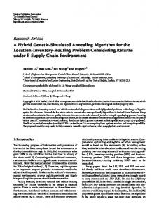
As can be seen, the annealing schedule consists of: 共1兲 The initial value of temperature T; 共2兲 a cooling function 共such as T = T · ␣ , 0 ⬍ ␣ ⬍ 1, i.e., between zero and one兲; 共3兲 the number of iterations to be performed at each temperature and 共4兲 a stopping criteria to terminate the algorithm. Extensive literature about simulated annealing can be seen from Eglese 共1990兲 and Koulamas et al. 共1994兲. Since SA provides a robust search as well as a near optimal solution in a reasonable time, this algorithm is employed as the solution technique for the BTRNDP. Before implementing the simulated annealing algorithm model, a set of potential routes, consisting of the whole solution space, has been generated by the ICRSGP. The objective of the simulated annealing algorithm presented here is to select an optimal set of routes from the candidate route set solution space with the total user, operator and unsatisfied demand cost being minimized. It should be pointed out that the SA algorithm presented here is solely oriented to the design of the transit networks from scratch. Details about applications of the SA algorithm on the redesign of transit networks can be seen in Fan 共2004兲. A flow chart that provides the SA algorithm-based solution framework for the BTRNDP is in Fig. 4. Note that the “neighborhood” for any route i is defined as the route right next to route i stored in the solution space. At the beginning of the SA implementation, the initial solutions are randomly generated. After the solution network route set is proposed, the search process is started. The network analysis procedure is called to assign the transit trips between each centroid node pair and determine the service frequencies on each route and evaluate the objective function for each proposed solution route set. For each iteration, if a solution route set is detected to improve over the current best one, the current best solution is updated. The new proposed solution sets are generated and evaluated in the same way. If convergence or the number of generations is satisfied, the iteration for a specific route set size completes. Then, the proposed solution route set size is incremented and same processes are repeated until the maximum route set size is reached. The best solution among all the route sets is adopted as the optimal solution to the BTRNDP for the current studied network.

Experimental Network and Numerical Results Example Network Configuration The simulated annealing based solution methodology is implemented through three experimental networks as a pilot study in our research. In this paper, one of these example networks is illustrated as shown in Fig. 5. This example network contains 28 travel demand zones and 65 road intersections. As noted before, the ICRSGP first considers the BTRNDP under the distribution node level. The network is processed as follows: 共1兲 The zonal demands are distributed the same way as the highway network demand; and 共2兲 if the same road link contains two or more demand distribution nodes from different zones, these distribution nodes are aggregated. After this preliminary process, 95 centroid distribution nodes, 160 nodes, and 418 arcs are obtained in this example network. The minimum and maximum route lengths are defined. In the example first phase, the ICRSGP generates 6,450 feasible routes whose distances satisfy these two route length constraints.

JOURNAL OF TRANSPORTATION ENGINEERING © ASCE / FEBRUARY 2006 / 127

Downloaded 25 Jul 2011 to 146.6.92.226. Redistribution subject to ASCE license or copyright. Visit http://www.ascelibrary.org

Fig. 4. SA implementation model for the BTRNDP

Numerical Results and Sensitivity Analyses As mentioned, the performance of the proposed simulated annealing algorithm model greatly depends upon the chosen parameters of the temperature, the stopping criteria 共i.e., the number of generations兲, the alpha value, and the repetition counter. Note that in essence, all the involved algorithm input parameters are continuous and can fall within a very large range. For example, the temperature and the number of generations can vary from 1 to positive infinity. One cannot try all combinations for all these parameters for any given weight set level for each objective

function component. Furthermore, even if one could find the optimal parameter set at a specific weight set level, this parameter set might not be optimal 共i.e., “best”兲 at another weight set level because we expect them to be problem and/or network size specific. However, it is also expected that similar 共i.e., general although might not be exactly the same兲 best input parameters can be obtained for different sized network 共as have been tested and proved using three different networks in our research兲. Therefore, for simplicity, several discrete values are chosen for each continuous parameter, and the optimal parameter set is decided

128 / JOURNAL OF TRANSPORTATION ENGINEERING © ASCE / FEBRUARY 2006

Downloaded 25 Jul 2011 to 146.6.92.226. Redistribution subject to ASCE license or copyright. Visit http://www.ascelibrary.org

Fig. 5. An example network with graphical representations for nodes, links, and routes

sequentially for the simulated annealing algorithm at a commonly used weight set level 共here 0.4, 0.4, and 0.2 is chosen for the weight of user cost, operator cost, and unsatisfied demand cost, respectively兲. For this purpose, the following sections present how the sensitivity analyses of these parameters are conducted using the designed network as an example. Effect of Temperature The effect of the initial temperature value is examined by varying this value from 100 to 10,000 and the result is given in Fig. 6共1兲. It can be seen from the figure that as the initial temperature increases, the objective function value changes unpredictably. It is also noted that the larger the chosen initial temperature, the more the computation time. When the initial temperature is chosen as 2,000, the least objective function value is achieved, suggesting that 2,000 should be chosen as the optimal initial temperature for the example network. Effect of Generations The effect of stopping criteria is investigated by choosing the number of generations ranging from 5 to 100 and the result is provided in Fig. 6共2兲. As can be seen, the least objective function value is achieved with 20 generations. Therefore, 20 is chosen as the optimal number of generations in terms of performance. Effect of Alpha Value The alpha value is introduced in the cooling function of SA to represent the ratio of the next temperature to previous one. The effect of the alpha value is also studied by varying this value from 0.1 to 0.9. The result shown in Fig. 6共3兲 indicates that 0.6 might be the optimal value and, as a result, it is recommended.

Effect of Repetition Counter The effect of repetition counter is examined by varying this value from 5 to 50 and the result is presented in Fig. 6共4兲. As can be seen, the least objective function value is achieved at 10, suggesting that the optimal repetition counter might be 10. Effect of Route Set Size At a commonly used and carefully chosen weight set level and the preferred parameter set as achieved above, the number of proposed routes in the solution network is varied from 1 to 10 and the effect of the route set size on several transit route network performance measures is provided in Fig. 7. As indicated, as the route set size increases, the solution improved initially because more transit demands are assigned to the network routes and unsatisfied demand costs decreases. However, the least objective function value is achieved with six routes for the studied network, and increases in the fleet size 共i.e., operator costs兲 produce underutilization of routes and does not result in an improved objective function value. Effect of Different Chosen Weights and Model Comparisons Different chosen weights for each component in the objective function can result in different solution network, as the results in Fig. 8 showed. To measure the solution quality using the presented SA for solving the BTRNDP, a genetic algorithm is used as a benchmark. 关The whole solution approach of genetic algorithm can be seen from Pattnaik et al. 共1998兲, and Fan and Machemehl 共2004兲.兴 In particular, it can be seen that at most of the unsatisfied demand cost weight level, the objective function values obtained from using SA model outperforms those from using genetic algorithm in each user cost weight set level. Furthermore, in terms of model performance, the SA is observed to be as stable as

JOURNAL OF TRANSPORTATION ENGINEERING © ASCE / FEBRUARY 2006 / 129

Downloaded 25 Jul 2011 to 146.6.92.226. Redistribution subject to ASCE license or copyright. Visit http://www.ascelibrary.org

Fig. 6. Numerical results and sensitivity analyses for the BTRNDP

the genetic algorithm 共as indicated by the similar pattern of the graphical variances兲. In addition to this example, two other experimental networks are also designed and tested for the performance of the SA and genetic algorithm. Numerical results showed that the SA algorithm is much better in the small network case and also no worse than the genetic algorithm in another case 共Fan 2004兲. This might suggest that the SA algorithm can be used as a potentially better 共at least a candidate as good as the genetic algorithm兲 approach than the genetic algorithm to solve the BTRNDP with fixed transit demand. However, to make this conclusion more convincing, further analyses for real world networks are still needed.

Conclusions This paper uses a simulated annealing algorithm for the first time to solve the optimal BTRNDP at the distribution node level. A multiobjective nonlinear mixed integer model is formulated for the BTRNDP. The proposed solution frameworks are presented.

Fig. 7. Performance measures versus route set size for the BTRNDP

A SA algorithm is employed as the solution method for finding an optimal set of routes from the huge solution space. The sensitivity analyses for the SA algorithm are conducted. The presented numerical results indicate that, as the route set size increases, the solution improved initially because more transit demands are assigned to the network routes and unsatisfied demand costs decreases. However, after the least objective function value is achieved under a certain amount set of routes for the studied network, the increase in the fleet size produce underutilization of routes and does not result in an improved objective function value. To measure the solution quality of the SA algorithm, a genetic algorithm is also used as a benchmark. Three experimental networks are designed and tested. Numerical results show that the proposed SA algorithm based model seems to outperform the genetic algorithm in most cases, suggesting that compared to

130 / JOURNAL OF TRANSPORTATION ENGINEERING © ASCE / FEBRUARY 2006

Downloaded 25 Jul 2011 to 146.6.92.226. Redistribution subject to ASCE license or copyright. Visit http://www.ascelibrary.org

Fig. 8. Sensitivity analyses results of different chosen weights for the BTRNDP and the comparisons of model performances between SA and genetic algorithm

the genetic algorithm, the SA is at least as good 共and potentially better兲 a candidate solution approach for the BTRNDP. Further application of this model to real world sized networks is under way.

Acknowledgments The writers appreciate the U.S. Department of Transportation, University Transportation Center through SWUTC to the Center for Transportation Research, The University of Texas at Austin for sponsoring this research through Project Nos. 167525 and 167824. They also want to thank two anonymous reviewers for their incisive and seasoned suggestions.

References Ahuja, R. K., Magnanti, T. L., and Orlin, J. B. 共1993兲. Network flows: Theory, algorithms, and applications, Prentice-Hall, Englewood Cliffs, N.J. Baaj, M. H., and Mahmassani, H. S. 共1991兲. “An AI-based approach for transit route system planning and design.” J. Adv. Transp., 25共2兲, 187–210.

Ceder, A., and Israeli, Y. 共1998兲. “User and operator perspective in transit network design.” Paper No. 980267, Proc., 77th Annual Meeting of TRB, Transportation Research Board, Washington, D.C. Ceder, A., and Wilson, N. H. M. 共1986兲. “Bus network design.” Transp. Res., Part B: Methodol., 20共4兲, 331–344. Chien S., Yang, Z., and Hou, E. 共2001兲. “A genetic algorithm approach for transit route planning and design.” J. Transp. Eng., 127共3兲, 200–207. Dubois, D., Bell, G., and Llibre, M. 共1979兲. “A set of methods in transportation network synthesis and analysis.” J. Oper. Res. Soc. 30, 797–808. Eglese, R. W. 共1990兲. “Simulated annealing: A tool for operational research.” Eur. J. Oper. Res., 46, 271–281. Fan, W. 共2004兲. “Optimal transit route network design problem: Algorithms, implementations, and numerical results.” PhD dissertation, Univ. of Texas at Austin, Austin, Tex. Fan, W., and Machemehl, R. B. 共2004兲. “A genetic algorithm approach for the transit route network design problem.” Proc., CSCE 2004, 5th Transportation Specialty Conf. Canadian Society for Civil Engineering, Saskatoon, Sask., Canada. Han, A. F., and Wilson N. 共1982兲. “The allocation of buses in heavily utilized networks with overlapping routes.” Transp. Res., Part B: Methodol., 16, 221–232. Hasselstrom, D. 共1981兲. “Public transportation planning—A mathematical programming approach.” PhD thesis, Dept. of Business

JOURNAL OF TRANSPORTATION ENGINEERING © ASCE / FEBRUARY 2006 / 131

Downloaded 25 Jul 2011 to 146.6.92.226. Redistribution subject to ASCE license or copyright. Visit http://www.ascelibrary.org

Administration, Univ. of Gothenburg, Gothenburg, Sweden. Koulamas, C., Antony, S. R., and Jaen, R. 共1994兲. “A survey of simulated annealing applications to operations research problems.” Omega, 22共1兲, 41–56. Lampkin, W., and Saalmans, P. D. 共1967兲. “The design of routes, service frequencies and schedules for a municipal bus undertaking: A case study.” Oper. Res. Q., 18, 375–397. LeBlanc, L. J. 共1988兲. “Transit system network design.” Transp. Res., Part B: Methodol. 22B共5兲, 383–390. National Cooperative Highway Research Program 共NCHRP兲. 共1980兲. “Bus route and schedule planning guidelines.” Synthesis of Highway Practice 69, Transportation Research Board, National Research Council, Washington, D.C. Newell, G. F. 共1979兲. “Some issues relating to the optimal design of bus routes.” Transp. Sci., 13共1兲, 20–35. Pattnaik, S. B., Mohan, S., and Tom, V. M. 共1998兲. “Urban bus transit network design using genetic algorithm.” J. Transp. Eng., 124共4兲, 368–375.

Rea, J. C. 共1971兲. “Designing urban transit systems: An approach to the rout-technology selection problem.” Rep. PB204881, Univ. of Washington, Seattle, Wash. Shih, M., Mahmassani, H. S., and Baaj M. 共1998a兲. “Trip assignment model for timed-transfer transit systems.” Transportation Research Record 1571, Transportation Research Board, Washington D.C., 24–30. Shih, M. C., Mahmassani, H. S., and Baaj, M. H. 共1998b兲. “A planning and design model for transit route networks with coordinated operations.” Proc., 77th Annual Meeting of TRB, Paper No. 980418, Transportation Research Board, Washington, D.C. Silman, L. A., Barzily, Z., and Passy, U. 共1974兲. “Planning the route system for urban buses.” Comput. Oper. Res., 1, 201–211. Van Nes, R., Hamerslag, R., and Immer, B. H. 共1988兲. “The design of public transport networks.” Transportation Research Record 1202, Transportation Research Board, Washington, D.C., 74–83. Yen, J. Y. 共1971兲. “Finding the K shortest loopless paths in a network.” Manage. Sci., 17共11兲, 712–716.

132 / JOURNAL OF TRANSPORTATION ENGINEERING © ASCE / FEBRUARY 2006

Downloaded 25 Jul 2011 to 146.6.92.226. Redistribution subject to ASCE license or copyright. Visit http://www.ascelibrary.org