A Knowledge-Based Simulated Annealing Algorithm to Multiple ...

Hindawi Publishing Corporation Journal of Applied Mathematics Volume 2013, Article ID 913450, 7 pages http://dx.doi.org/10.1155/2013/913450

Research Article A Knowledge-Based Simulated Annealing Algorithm to Multiple Satellites Mission Planning Problems Da-Wei Jin1 and Li-Ning Xing2 1 2

Information and Safety School, Zhongnan University of Economic and Law, Wuhan 430073, China College of Information System and Management, National University of Defense Technology, Changsha 410073, China

Correspondence should be addressed to Li-Ning Xing; [email protected] Received 21 September 2013; Accepted 5 November 2013 Academic Editor: Zhongxiao Jia Copyright © 2013 D.-W. Jin and L.-N. Xing. This is an open access article distributed under the Creative Commons Attribution License, which permits unrestricted use, distribution, and reproduction in any medium, provided the original work is properly cited. The multiple satellites mission planning is a complex combination optimization problem. A knowledge-based simulated annealing algorithm is proposed to the multiple satellites mission planning problems. The experimental results suggest that the proposed algorithm is effective to the given problem. The knowledge-based simulated annealing method will provide a useful reference for the improvement of existing optimization approaches.

1. Introduction The imaging satellite plays a significant role in various fields such as the disaster prevention and environmental protection and attracts great attention of many scholars in the world [1, 2]. Although the number of satellites in orbit is increasing, the imaging satellite resources are still limited compared with the rapid growing imaging requirements [3, 4]. To improve the performance of satellite resources, the appropriate mathematical models and software tools must be employed to realize a better management and allocation of satellite resources [5, 6]. With the development of aerospace industry, the number and classification of imaging satellites are increasing. Also, both the number and the category of imaging requirements are largely increased [7]. It is very necessary to make a comprehensive scheduling of multiple imaging satellites [8, 9]. Therefore, this paper proposes a novel method to deal with the multiple satellites mission planning problem [10, 11]. The motivation of this work can be summarized as follows. At first, the multiple satellites mission planning is a classical combination optimization problem and it is very urgent to develop some new methods to deal with this problem. At second, the interaction between evolution and learning is more popular than before, so a knowledge-based

simulated annealing algorithm is designed and implemented according to this fashion.

2. Multiple Satellites Mission Planning Problems The multiple satellites mission planning problem can be summarized as follows. Under the conditions of satisfying the resource constraints and imaging requirements, make a comprehensive scheduling of spot targets and regional targets, allocate satellite resources and working time for each target, and develop an optimized observation plan to maximize the summation of priority of completed targets. There are two subproblems to be solved in this problem. One is how to make a comprehensive scheduling of spot targets and regional targets, based on which the other one is how to optimize the observation plan of satellite resources. The multiple satellites mission planning is a complex combination optimization problem. 2.1. Hypothesis (1) There is only one sensor in each satellite. In fact, if there are multiple sensors in one satellite, then this

2

Journal of Applied Mathematics satellite can be divided into multiple satellites with one sensor. For this reason, both the sensor 𝑠𝑖 and the satellite 𝑠𝑖 have the same meaning. (2) The regional target can be divided into multiple atomic tasks. In fact, a spot target just is one atomic task. In this paper, the atomic task 𝑜𝑖𝑗𝑘V means the Vth subtask of task 𝑡𝑗 which can be observed in the 𝑘th time window of satellite 𝑠𝑖 . The regional target 𝑡𝑗 is divided into the following sets: 𝑁𝑆 𝑁𝑖𝑗 𝑁𝑖𝑗𝑘

𝑂𝑗 = ⋃ ⋃ ⋃ 𝑜𝑖𝑗𝑘V ,

2.3. Outputs. In the multiple satellites mission planning problem, the outputs (decision variables) can be summarized as follows: 1, { { 𝑙 ={ 𝑥𝑖𝑗𝑘V { {0,

The atomic task 𝑜𝑖𝑗𝑘V was executed in the 𝑙th composite tasks of satellite 𝑠𝑖 Otherwise.

2.4. Objectives. The objective of this problem is to maximize the priority summation of fulfilled tasks. That is, max 𝐽 = 𝐶Spot + 𝐶Polygon ,

(1)

𝑖=1 𝑘=1 V=1

where 𝑁𝑆 denotes the number of satellites, 𝑁𝑖𝑗 denotes the number of visible time windows about sensor 𝑠𝑖 and target 𝑡𝑗 , and 𝑁𝑖𝑗𝑘 denotes the number of atomic tasks which can be observed in the 𝑘th time window of satellite 𝑠𝑖 . (3) In order to improve the performance of imaging resources, multiple atomic tasks are integrated into one composite task, which can be observed at one time. 2.2. Inputs (1) The number of satellites is 𝑁𝑆 . Span𝑖 denotes the longest working time of satellite 𝑠𝑖 within one single booting. (2) 𝑀𝑖 and 𝑃𝑖 denote the maximum of storage capacity and energy of satellite 𝑠𝑖 , 𝑚𝑖 , and 𝑝𝑖 refer to the storage and energy consumption of satellite 𝑠𝑖 for observation in unit time. (3) 𝑅𝑖 denotes the maximum number of side-view imaging in each circle, 𝜗𝑖 is the swaying speed of satellite 𝑠𝑖 (degree per second), 𝜌𝑖 refers to the energy consumption of swaying in each degree, 𝑑𝑖 is the settling time of swaying of satellite 𝑠𝑖 . (4) The number of tasks is 𝑁𝑇 . Suppose the first ℎ targets are spot ones, and the last 𝑁𝑇 − ℎ targets are regional ones. LP𝑖 means the priority of target 𝑖. 𝑁 {V𝑤𝑖𝑗1 , V𝑤𝑖𝑗2 , . . . , V𝑤𝑖𝑗 𝑖𝑗 }

(5) 𝑉𝑊𝑖𝑗 = denotes the set of time windows about sensor 𝑠𝑖 and target 𝑡𝑗 , and 𝑁𝑖𝑗 is the total number of visible time windows about sensor 𝑠𝑖 and target 𝑡𝑗 . (6) 𝑤𝑠𝑖𝑗𝑘V , 𝑤𝑒𝑖𝑗𝑘V , and 𝑔𝑖𝑗𝑘V refer to the starting time, ending time, and observation angle of atomic task 𝑜𝑖𝑗𝑘V , respectively. (7) 𝑏𝑖𝑙 denotes the 𝑙th composite task of satellite 𝑠𝑖 , while 𝑤𝑠𝑖𝑙 , 𝑤𝑒𝑖𝑙 , and 𝑔𝑖𝑙 refer to the starting time, ending time, and observation angle of composite task 𝑏𝑖𝑙 . (8) 𝐵𝑖 = {𝑏𝑖1 , 𝑏𝑖2 , . . . , 𝑏𝑖𝑁𝐵 } denotes the set of composite 𝑖 tasks of satellite 𝑠𝑖 , in which 𝑁𝐵𝑖 is the number of composite tasks.

(2)

(3)

where 𝐶Spot denotes the priority summation of spot targets, and it is ℎ

𝐶Spot = ∑ 𝐶Spot (𝑡𝑗 ) 𝑗=1

(4)

ℎ 𝑁𝑆 𝑁𝑖𝑗 𝑁𝐵𝑗

𝑙 = ∑ ∑ ∑ ∑ 𝑥𝑖𝑗𝑘1 × LP𝑗 . 𝑗=1 𝑖=1 𝑘=1 𝑙=1

𝐶Polygon means the priority summation of regional targets. This computation process is a little complex. At first, we should compute the overlap area between the multiple observed atomic tasks and regional target 𝑡𝑗 . That is, 𝑁𝑆 𝑁𝑖𝑗 𝑁𝑖𝑗𝑘 𝑁𝐵𝑖

𝑙 𝜓 (𝑜𝑖𝑗𝑘V )) ⋂ 𝜓 (𝑡𝑗 ) . 𝑆Polygon = (⋃ ⋃ ⋃ ⋃ 𝑥𝑖𝑗𝑘V

(5)

𝑖=1 𝑘=1 V=1 𝑙=1

Here, 𝜓(𝑜𝑖𝑗𝑘V ) denotes the polygon area of atomic task 𝑜𝑖𝑗𝑘V , ∩ denotes the intersection operation of multiple sets, 𝜓(𝑡𝑗 ) denotes the polygon area of regional target 𝑡𝑗 , and ∪ denotes the union operation of different sets. At second, we should compute the coverage rate of each regional target. It is Cover (𝑡𝑗 ) =

𝑓 (𝑆Polygon ) 𝑓 (𝑡𝑗 )

,

(6)

where 𝑓(𝑆Polygon ) denotes the proportion of polygon area 𝑆Polygon , and 𝑓(𝑡𝑗 ) denotes the proportion of regional target 𝑡𝑗 . In total, the priority summation of regional targets can be computed as follows: 𝑁𝑇

𝐶Polygon = ∑ [Cover (𝑡𝑗 ) × LP𝑗 ] .

(7)

𝑗=ℎ+1

2.5. Constraints (1) Uniqueness constraint on spot targets; that is, each spot target can only be observed once: 𝑁𝑆 𝑁𝑖𝑗 𝑁𝐵𝑗

𝑙 ≤ 1, ∑ ∑ ∑ 𝑥𝑖𝑗𝑘1 𝑖=1 𝑘=1 𝑙=1

∀𝑗 = 1, . . . , ℎ.

(8)

Journal of Applied Mathematics

3

(2) Conversion time constraints between composite tasks, it is 󵄨 󵄨󵄨 󵄨󵄨𝑔𝑖𝑙 − 𝑔𝑖(𝑙+1) 󵄨󵄨󵄨 + 𝑑𝑖 ≤ 𝑤𝑠𝑖(𝑙+1) , 𝑤𝑒𝑖𝑙 + 𝜗𝑖 (9) ∀𝑖 = 1, . . . , 𝑁𝑆 ; 𝑙 = 1, . . . , 𝑁𝐵𝑖 − 1. Each composite task corresponds to an observation activity of the satellite, and every two composite tasks must satisfy the corresponding conversion time constraint. The conversion time include the rotation time and settling time of the sway. (3) Storage constraints of the satellite: 𝑁𝐵𝑖

∑ (𝑤𝑒𝑖𝑙 − 𝑤𝑠𝑖𝑙 ) 𝑚𝑖 ≤ 𝑀𝑖 , 𝑙=1

∀𝑖 = 1, . . . , 𝑁𝑆 .

(10)

(4) Energy constraints of the satellite: 𝑁𝐵𝑖

𝑁𝐵𝑖 −1

𝑙=1

𝑙=1

󵄨 󵄨 ∑ (𝑤𝑒𝑖𝑙 − 𝑤𝑠𝑖𝑙 ) 𝑝𝑖 + ∑ 󵄨󵄨󵄨𝑔𝑖(𝑙+1) − 𝑔𝑖𝑙 󵄨󵄨󵄨 𝜌𝑖 ≤ 𝑃𝑖 ,

(11)

∀𝑖 = 1, . . . , 𝑁𝑆 . The satellites usually consume some energy during the imaging and swaying process, so the corresponding energy consumption can be represented in a function about the observation time of satellites and sensor’s swaying. The energy consumption should not exceed the largest energy limitation. (5) Constraint on the maximum number of side-view imaging in a single circle. We can obtain the identifier of orbit circles according to the starting time and ending time of observation activities and then verify this constraint. Suppose the orbit set of satellite 𝑠𝑖 is Orbit𝑖 = {orbit𝑖1 , orbit𝑖2 , . . . , orbit𝑖𝑁𝑂 } 𝑖

(12)

in which 𝑁𝑂𝑖 is the number of orbits, and orbit𝑖𝑟 refers to orbit 𝑟 of satellite 𝑠𝑖 . Given that orbit𝑖𝑟 contains 𝑁𝑖𝑟 composite tasks {𝑏𝑖𝑟1 , 𝑏𝑖𝑟2 , . . . , 𝑏𝑖𝑟𝑁 }, 𝑖𝑟

𝑁𝑖𝑟 ≤ 𝑅𝑖 ,

∀𝑖 = 1, . . . , 𝑁𝑆 , 𝑟 = 1, . . . , 𝑁𝑂𝑖 .

(13)

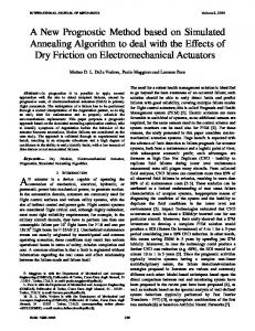
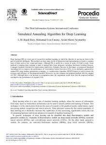
3. The Proposed Approach In the existing intelligent optimization methods, they have not involved the effective management (i.e., learning, storage, and utilization) to domain knowledge of practical problems, and thus they cannot effectively obtain the optimal solution of optimization problems. Based on our knowledge, the complex optimization problem can be solved through learning some related knowledge from the optimization process and then employing it to guide the subsequent optimization process. In this paper, we mainly focus on the explicit

knowledge, namely, the knowledge that can be definitely expressed. All the explicit knowledge can be expressed and stored through computer language and updated and adopted by other models. In this paper, the knowledge-based simulated annealing algorithm is defined as a hybrid approach which effectively combines the simulated annealing model and knowledge model, in which the simulated annealing model searches the solution space of optimization problems by “neighborhood search” strategy, and the knowledge model learns useful knowledge from the optimization process and then uses it to guide the subsequent optimization process. The knowledge-based simulated annealing algorithm employs the modeling idea of integrating the knowledge model and the simulated annealing model. Its basic framework is shown in Figure 1. The working mechanism of knowledge-based simulated annealing algorithm is shown in Figure 2. The top illustrates the optimization process of simulated annealing algorithm: search the feasible space of optimization problems through the “neighborhood search” strategy and then converge to the near-optimal solution through continually iterations. And the bottom shows the effect of knowledge model: learn the useful knowledge from the early optimization process and then apply it to guide the subsequent optimization process. During the early operation process of knowledge-based simulated annealing algorithm, due to that the available samples are not sufficient, so the reliability of learned knowledge is not high, and the guidance to optimization process is not distinct. However, with the advance of iterations, the reliability of learned knowledge is higher than before, and the guidance to optimization process is more distinct. Compared with traditional simulated annealing algorithm, with the help of knowledge model, the knowledge-based simulated annealing algorithm can either converge to a satisfactory solution more quickly or converge to a satisfactory solution with higher quality. 3.1. Knowledge Definition, Learning, and Application (1) Operator Knowledge. Usually, different operators have different application scopes. When solving practical problems, a single operator may be more effective to some problems than to others. Therefore, it is very difficult to find out a general operator that can solve all kinds of practical problems effectively. In order to improve the performance of simulated annealing algorithm, we can adopt several kinds of operators for different operations in simulated annealing algorithm, with the hope of trying to mine some operators that can effectively solve the present problem. When an operator is employed to one operation, suppose the original individual set is 𝐶𝐵 and the newly generated individual set is 𝐶𝐴 , and if the optimal individual in 𝐶𝐴 is better than that in 𝐶𝐵 , then the present operation is considered to be successful. The optimization performance of one operator can be defined as the number of successful operations realized by the given operator. Operator knowledge mainly

4

Journal of Applied Mathematics Knowledge-based simulated annealing algorithm

Learn useful knowledge from the optimization process

Simulated annealing model

Knowledge model

Apply the knowledge to guide the subsequent optimization process

Figure 1: The basic framework of knowledge-based simulated annealing algorithm.

The optimization process of simulated annealing algorithm The first iteration

The second iteration

The third iteration

···

The (k − 1)th iteration

The Kth iteration

Adopt the acquired knowledge to guide subsequent optimization process

Acquire knowledge from early optimization process Acquire knowledge from early optimization process Acquire knowledge from early optimization process Knowledge model (the representation, acquisition, storage, and application of knowledge)

Figure 2: The operation mechanism of knowledge-based simulated annealing algorithm.

refers to the accumulated knowledge for the optimization performance of various operators. The simple case for extraction and application of operator knowledge is displayed as follows. Suppose there are three operators in the simulated annealing algorithm, if the current operation implemented by the 𝑘th operator is successful, then the optimization performance 𝑁(𝑘) of the 𝑘th operator will be added by one. During the next operation, the selection probability for each operator will be calculated according to the following formula: 𝑃 (𝑖) =

𝑁 (𝑖)

∑3𝑖=1

𝑁 (𝑖)

,

(14)

where 𝑃(𝑖) denotes the probability that the 𝑖th operator is selected for the operation. (2) Parameter Knowledge. One simple and easy method to improve the optimization performance of simulated annealing algorithm is to adjust the parameter values dynamically during the optimization process. To lower the sensitivity of parameters to experimental results, we employ several different parameter combinations to develop the evolution process and decide the parameter combination selected for the next iteration according to their optimization performance. After a single iteration, if the global optimal solution has been improved, then it is a successful iteration. In the process

of solving current cases, the number of successful iterations obtained by the given parameter combination is regarded as its optimization performance. Parameter knowledge mainly refers to the accumulated knowledge of the optimization performance for various parameter combinations. During the initialization stage, the orthogonal method can be adopted to generate different parameter combinations and all their optimization performance is initialized to 1. Before any iteration of simulated annealing algorithm, a parameter combination will be selected stochastically from several parameter combinations through roulette selection (based on the optimization performance of parameter combinations) as the parameter of current iteration. If the global optimal solution has been improved in this iteration, then the optimization performance value of the parameter combination used in this iteration will be increased. 3.2. The Available Neighborhood Structures. The following neighborhood structures have been designed based on the basic ones and passed the constraint checking of the basic neighborhood structure, thus greatly simplifying the optimization calculation process. (1) Arrange. The scheduling of imaging satellites for composing tasks usually involves the task arrangement which is performed through composing or inserting the contained

Journal of Applied Mathematics

(2) Relocate. This kind of neighborhood can reallocate the satellite resource and time windows of tasks. There are several time windows about satellites and tasks, so we can reallocate time windows for the task as to the same satellite. Two kinds of operations are involved here: one is to reallocate the task to different time windows about the same satellite and the other is to reallocate the task to another satellite. The relocating aims to increase the chance of arranging other tasks through adjusting the satellite resource and time windows of tasks. (3) Swap. This neighborhood aims to exchange two tasks. About parallel scheduling problems, three kinds of neighborhood structures for task exchange are mentioned: the exchange between two tasks with the same resource (exchanging the execution order); the exchange between two tasks with different resources; the exchange between the scheduled tasks and unscheduled ones. To the multiple satellites mission planning problem, the relevant experiments indicate that the first two exchanges are unsuccessful. Therefore, this paper adopts the third kind of neighborhood structure for task exchange, namely, to exchange tasks under the real satellite resource and the virtual one. (4) Sample. Random sampling neighborhood is a special measure adopted to handle large-scale neighborhood effectively. It is not a new neighborhood structure itself, but a method to generate new neighbourhood structures through sampling the existing ones randomly. To be specific, before each move, random sampling neighbourhood will sample all neighbors generated by the given neighbourhood structure, so as to limit the move to part of the sampled neighbourhood, and the proportion of sampling is usually specified in advance upon requirements. Among the designs of neighbourhood structure, the arrangement of neighbourhood is designed to implement the insertion and composition operations among atomic tasks in which the task composition is preferred, and it is a kind of improved neighbourhood; the neighbourhood relocation and swap disturb the solutions, respectively, through adjusting the resources and time windows of the task as well as exchanging the scheduled tasks with unscheduled ones, and they belong to a regulative neighbourhood which can increase the chance to arrange other tasks after the relocation and swap of tasks, so they should be tried on all the unfinished tasks.

4. Experimental Results Six sets of even-distributed targets are generated, respectively, with the number of 100, 200, 300, 400, 500, and 600. Based on a different number of satellites, several test cases are then constructed for each set of targets. Each case will be

1200 1000 Optimization performance

atomic tasks. Neighborhood composition is preferred in the arrangement of atomic tasks, and the insertion operation is adopted only when atomic tasks cannot be composed or the task has not been finished, which contributes to the observation composition of much more tasks and helps to arrange more tasks.

5

800 600 400 200 0

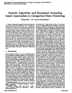
100 × 2 100 × 4 100 × 6 200 × 2 200 × 4 200 × 6 Testing examples (number of tasks × number of satellites) HM SSAA KSSA

Figure 3: Experimental results in optimization performance of small scale testing examples.

calculated for fifty times and the comparison will be made on the averages of the results to avoid the influence of randomness. To validate the performance of this algorithm, the Heuristic Method (HM) and the Standard Simulated Annealing Algorithm (SSAA) are employed to be compared with the Knowledge-Based Simulated Annealing Algorithm (KSAA). 4.1. Experimental Results of Small Scale Testing Examples. Six small scale testing examples (100 × 2, 100 × 4, 100 × 6, 200 × 2, 200 × 4, 200 × 6) are applied to test the performance of different algorithms. Experimental results of small scale testing examples are displayed in Figures 3 and 4. Experimental results in Figure 3 suggest that there is no remarkable difference in optimization performance among HM, SSAA, and KSSA. Experimental results in Figure 4 suggest that the computational time of SSAA and KSSA is little larger than that of HM. Also, there is no distinct difference in computational time between SSAA and KSSA. Since SSAA and KSSA are all intelligent optimization approaches, so the computational time of SSAA and KSSA is larger than that of HM. 4.2. Experimental Results of Medium Scale Testing Examples. Six medium scale testing examples (300 × 2, 300 × 4, 300 ×6, 400×2, 400×4, 400×6) are applied to test the performance of different algorithms. Experimental results of medium scale testing examples are displayed in Figures 5 and 6. Experimental results in Figure 5 suggest that there is no significant difference in optimization performance among SSAA and KSSA, but the optimization performance of SSAA and KSSA is better than that of HM. Since SSAA and KSSA are all intelligent optimization approaches, so the optimization performance of SSAA and KSSA should be

6

Journal of Applied Mathematics 35

300 250

25

Computational time (s)

Computational time (s)

30

20 15 10 5 0

200 150 100 50

100 × 2 100 × 4 100 × 6 200 × 2 200 × 4 200 × 6 Testing examples (number of tasks × number of satellites)

0 300 × 2

300 × 4

300 × 6

400 × 2

400 × 4

400 × 6

Testing examples (number of tasks × number of satellites)

HM SSAA KSSA

Figure 4: Experimental results in computational time of small scale testing examples.

HM SSAA KSSA

Figure 6: Experimental results in computational time of medium scale testing examples.

2500

2000

3500 Optimization performance

Optimization performance

4000

1500

1000

500

3000 2500 2000 1500 1000 500

0

300 × 2

300 × 4

300 × 6

400 × 2

400 × 4

400 × 6

Testing examples (number of tasks × number of satellites)

HM SSAA KSSA

Figure 5: Experimental results in optimization performance of medium scale testing examples.

better than that of HM, and the experimental result indicates this viewpoint. Experimental results in Figure 6 suggest that the computational time of SSAA and KSSA is little larger than that of HM. Also, there is no distinct difference in computational time between SSAA and KSSA. 4.3. Experimental Results of Large Scale Testing Examples. Six large scale testing examples (500 × 4, 500 × 6, 500 × 8, 600 × 4, 600 × 6, 600 × 8) are applied to test the performance of different algorithms. The experimental results of large scale testing examples are displayed in Figures 7 and 8.

0

500 × 4

500 × 6

500 × 8

600 × 4

600 × 6

600 × 8

Testing examples (number of tasks × number of satellites)

HM SSAA KSSA

Figure 7: Experimental results in optimization performance of large scale testing examples.

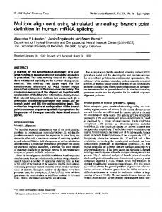
Experimental results in Figure 7 suggest that the optimization performance of SSAA is better than that of HM, and the optimization performance of KSAA is better than that of SSAA. Since SSAA is an intelligent optimization approach, so the optimization performance of SSAA should be better than that of HM, and experimental results indicate this viewpoint. At the same time, KSAA extended the learning and guidance function based on the SSAA, so its performance should be better than that of SSAA, and experimental results validate this opinion. Experimental results in Figure 8 suggest that

Journal of Applied Mathematics

Acknowledgments

1400

The authors would like to thank the reviewers for the valuable comments and constructive suggestions. they also would like to thank the editor-in-chief, associate editor and editors for helpful suggestions. This work is supported by the National Natural Science Foundation of China (nos. 71101150, 71071156, and 71331008), Program for New Century Excellent Talents in University, the Ministry of Education in China (MOE) Project of Humanities and Social Sciences (no. 12YJC630078).

1200 Computational time (s)

7

1000 800 600 400

References

200 0 500 × 4 500 × 6 500 × 8 600 × 4 600 × 6 600 × 8 Testing examples (number of tasks × number of satellites) HM SSAA KSSA

Figure 8: Experimental results in computational time of large scale testing examples.

the computational time of SSAA is larger than that of HM, and the computational time of KSAA is larger than that of SSAA. Since SSAA is an intelligent optimization approach, so it needs more computation cost than that of HM to deal with large scale testing examples. Also, the number of modules in KSSA is more than that in SSAA, so it needs more computation cost than that of SSAA to deal with large scale testing examples.

5. Conclusions The innovation of this paper lies in that it has established a multisatellite mission planning model based on the constraint satisfaction and proposed a knowledge-based simulated annealing algorithm to solve multisatellite mission planning problems, which has been proved effective in the relevant experiment. The future research directions can be summarized as follows. (1) Extend the types of knowledge. Extracting the experiential knowledge of experts to multiple satellites mission planning problems, we could employ this knowledge to guide the optimization process effectively so as to enhance optimization efficiency as much as possible. (2) Adopt new knowledge mining techniques. We should consider employing advanced knowledge mining through machine learning or data mining to obtain useful knowledge from the optimization process.

Conflict of Interests The authors declare no conflict of interests.

[1] V. Gerard and L. Michel, “Planning activities for Earth watching and observing satellites and constellations,” in Proceedings of the 16th International Conference on Automated Planning and Scheduling (ICAPS ’06), Cumbria, UK, 2006. [2] F. N. Kucinskis and M. G. V. Ferreira, “Planning on-board satellites for the goal-based operations for space missions,” IEEE Latin America Transactions, vol. 11, no. 4, pp. 1110–1120, 2013. [3] A. Manzak and H. Goksu, “Application of Very Fast Simulated Reannealing (VFSR) to low power design,” in Proceedings of the 5th International Workshop on Embedded Computer Systems: Architectures, Modeling, and Simulation (SAMOS ’05), pp. 308– 313, Springer, Berlin, Germany, July 2005. [4] Z. Y. Lian, Y. Wang, Y. J. Tan et al., “Integration solving framework for global navigation satellite system planning and scheduling problem,” Disaster Advanced, vol. 6, no. 1, pp. 330– 336, 2013. [5] S. Rojanasoonthon and J. Bard, “A GRASP for parallel machine scheduling with time windows,” INFORMS Journal on Computing, vol. 17, no. 1, pp. 32–51, 2005. [6] R. J. He and L. N. Xing, “A learnable ant colony optimization to the mission planning of multiple satellites,” Research Journal of Chemistry and Environment, vol. 16, no. S2, pp. 18–26, 2012. [7] B. Suman and P. Kumar, “A survey of simulated annealing as a tool for single and multiobjective optimization,” Journal of the Operational Research Society, vol. 57, no. 10, pp. 1143–1160, 2006. [8] A. Globus, J. Crawford, J. Lohn, and A. Pryor, “A comparison of techniques for scheduling earth observing satellites,” in Proceedings of the 19th National Conference on Artificial Intelligence (AAAI-2004): Sixteenth Innovative Applications of Artificial Intelligence Conference (IAAI ’04), pp. 836–843, July 2004. [9] D. A. Knapp, D. S. Roffman, and W. J. Cooper, “Growth of a pharmacy school through planning, cooperation, and establishment of a satellite campus,” American Journal of Pharmaceutical Education, vol. 73, no. 6, article 102, 2009. [10] B. Sudarshan and D. R. Nikil, “Very fast simulated annealing for HW-SW partitioning,” Tech. Rep. CECS-TR-04-17. UC, Irvine, 2004. [11] C. Wang, J. Li, N. Jing, J. Wang, and H. Chen, “A distributed cooperative dynamic task planning algorithm for multiple satellites based on multi-agent hybrid learning,” Chinese Journal of Aeronautics, vol. 24, no. 4, pp. 493–505, 2011.

Advances in

Operations Research Hindawi Publishing Corporation http://www.hindawi.com

Volume 2014

Advances in

Decision Sciences Hindawi Publishing Corporation http://www.hindawi.com

Volume 2014

Journal of

Applied Mathematics

Algebra

Hindawi Publishing Corporation http://www.hindawi.com

Hindawi Publishing Corporation http://www.hindawi.com

Volume 2014

Journal of

Probability and Statistics Volume 2014

The Scientific World Journal Hindawi Publishing Corporation http://www.hindawi.com

Hindawi Publishing Corporation http://www.hindawi.com

Volume 2014

International Journal of

Differential Equations Hindawi Publishing Corporation http://www.hindawi.com

Volume 2014

Volume 2014

Submit your manuscripts at http://www.hindawi.com International Journal of

Advances in

Combinatorics Hindawi Publishing Corporation http://www.hindawi.com

Mathematical Physics Hindawi Publishing Corporation http://www.hindawi.com

Volume 2014

Journal of

Complex Analysis Hindawi Publishing Corporation http://www.hindawi.com

Volume 2014

International Journal of Mathematics and Mathematical Sciences

Mathematical Problems in Engineering

Journal of

Mathematics Hindawi Publishing Corporation http://www.hindawi.com

Volume 2014

Hindawi Publishing Corporation http://www.hindawi.com

Volume 2014

Volume 2014

Hindawi Publishing Corporation http://www.hindawi.com

Volume 2014

Discrete Mathematics

Journal of

Volume 2014

Hindawi Publishing Corporation http://www.hindawi.com

Discrete Dynamics in Nature and Society

Journal of

Function Spaces Hindawi Publishing Corporation http://www.hindawi.com

Abstract and Applied Analysis

Volume 2014

Hindawi Publishing Corporation http://www.hindawi.com

Volume 2014

Hindawi Publishing Corporation http://www.hindawi.com

Volume 2014

International Journal of

Journal of

Stochastic Analysis

Optimization

Hindawi Publishing Corporation http://www.hindawi.com

Hindawi Publishing Corporation http://www.hindawi.com

Volume 2014

Volume 2014