Jun 22, 2009 - Sub-clauses Deduction. (full paper). Sylvain Darras, Gilles Dequen, Laure Devendeville. Laria â Universit de Picardie Jules Vernes. {darras ...
Author manuscript, published in "11th International Conference on Principles and Practice of Constraint Programming (CP'05), Sitges : Spain (2005)"
Using Boolean Constraint Propagation for Sub-clauses Deduction (full paper)
hal-00396436, version 1 - 22 Jun 2009
Sylvain Darras, Gilles Dequen, Laure Devendeville Laria – Universit de Picardie Jules Vernes {darras,dequen,devendeville}@laria.univ-picardie.fr
Bertrand Mazure, Richard Ostrowski, Lakhdar Sa¨ıs CRIL CNRS – Universit d’Artois rue Jean Souvraz SP-18 F-62307 Lens Cedex France {ostrowski,mazure,sais}@cril.univ-artois.fr
Abstract Boolean Constraint Propagation (BCP) is recognized as one of the most useful technique for efficient satisfiability checking. In this paper a new extension of the scope of boolean constraint propagation is proposed. It makes an original use of BCP to achieve further reduction of boolean formulas. Considering the implication graph generated by the constraint propagation process as a resolution tree, sub-clauses from the original formula can be deduced. Then, we show how such extension can be grafted to modern SAT solvers where BCP is maintained at each step of the search tree. Preliminary results of “Zchaff” - the state of the art SAT solver - augmented with extended BCP, show the great potential of our approach with respect to certain classes of SAT instances. Keywords: SAT, Boolean Constraint Propagation, reasoning and search, learning, subsumption.
1 Introduction Recent impressive progress in the practical resolution of hard and large SAT instances allows real-world problems that are encoded in propositional clausal normal form (CNF) to be addressed (e.g. [7, 8, 11, 2]). Many benchmarks have been proposed and regular competitions (e.g. Dimacs’93, Beijing’96, SAT’01-04) are organized around
1
hal-00396436, version 1 - 22 Jun 2009
these specific SAT instances, which are expected to encode structural knowledge at least to some extent. The huge size of the real-world SAT instances currently in the scope of modern SAT solvers such as Zchaff [12], allows to consider practical applications. Such a progress shows us that instances with worst case complexity behavior appears rarely in practice. Indeed, instances from practical applications contain some structures that can benefit to SAT solvers. One of them is that clauses share more common variables comparatively to random instances. For example, the clauses encoding the boolean formula x1 ∧ x2 → y1 ∧ y2 ∧ · · · ∧ yn share the two boolean variables x1 and x2 . In other words, many common sub-clauses results from the elimination of boolean connectives (e.g. ∨, ∧, ↔). One can see that after assigning the value f alse to yi the other clauses become redundant and can be eliminated by subsumption using the clause ¬x1 ∨ ¬x2 . Our intuition is that when considering large SAT instances at each step of the search process, many clauses become redundant and some sub-clauses might be deduced and then decrease the size of the formula. Considering large SAT instances at each step of DPL search process, our intution is that some sub clauses can be deduced with the resolution rule and then useless according to the subsumption rule. This idea can be maintened at each node of search tree of the formula and then produce some formulas where the number of clauses cannot be greater than the initial one and where for a given clause become redondant and then useless according to the subsumption rule. On the other hand, some subclauses can be deduced according to the resolution rule The main objective of this paper is to show how such structural knowledge can be exploited during search. We focus on sub-clauses deductions that might help reducing the formula to its “real” size and give rise to a constant space complexity approach. Boolean constraint propagation (or unit propagation), applying in all efficient DPLL implentations [9, 4, 12] can be considered as a restricted form of resolution and as a special case of subsumption rule. It is recognized as one of the most important paradigm for efficient satisfiability checking. Indeed, most of modern SAT solver are based on the well known DavisPutnam-Logemann-Loveland (DPLL) procedure [3] where BCP is maintained at each step of the search process. On many SAT instances, a major part of the search space (about 90% ) is achieved using BCP. This important role has motivated many works on efficient implementation of BCP (e.g. Zchaff) and on extending its practical use. Among others, many simplification techniques (e.g. [5, 1]), variable ordering heuristics (e.g. [9, 4]), conflict analysis scheme (e.g. [10, 12]), functional dependencies deduction (e.g. [6]) are based on BCP. In this paper, a new extension of the scope of boolean constraint propagation is proposed. It makes an original use of BCP to achieve further reduction of boolean formulas. More precisely, the constraint graph generated by the boolean constraint propagation process can be mapped to a resolution tree which encodes clauses of the original formula and new resolvent. The set of such possible resolvent can have an exponential size in the worst case w.r.t. the set of clauses encoded in the constraint graph. To avoid such a drawback, the approach proposed in this paper considers only a relevant set of resolvent leading to a polynomial time and constant space complexity approach. Then, we show how such an extension can be grafted to modern SAT solvers. 2
The paper is organized as follows. After some preliminary definitions, relations between resolution and boolean constraint propagation are discussed. Then a constant space complexity BCP-based approach for sub-clauses deduction is proposed, allowing the formula to be reduced. Its dynamic integration in SAT solvers is presented and some preliminary experimental results showing the interest of the proposed approach are provided. Finally, promising paths for future research are discussed in the conclusion.
hal-00396436, version 1 - 22 Jun 2009
2 Definitions and preliminaries A CNF formula Σ is a set (interpreted as a conjunction) of clauses, where a clause is a set (interpreted as a disjunction) of literals. A literal is a positive or negative propositional variable. We note var(Σ) (resp. lit(Σ)) the set of variables (resp. literals) occurring in Σ. A unit clause is a clause containing a single literal called unit literal. A binary clause contains two literals associated with two distinct variables. A clause containing literals of distinct variables is called fundamental. It is called tautological P when it contains two opposite literals. The size of the formula Σ is given by |Σ| = c∈Σ |c|, where |c| is the number of literals in c. In the following, we use formula (resp. variable) instead of CNF formula (resp. propositional variable). In addition to the set-based notations, we define the negation of a set A of literals as the set A¯ of the corresponding opposite literals. We note A∨ (respectively A∧ ) the disjunction (resp. conjunction) of all literals of A. An interpretation of a formula Σ is an assignment of truth values {true, f alse} to its variables. It is called partial interpretation if only a subset of variables of var(Σ) are assigned. A model of a formula is an interpretation that satisfies the formula. Accordingly, SAT consists in finding a model of a formula when such a model exists or in proving that such a model does not exist. A formula ψ is a logical consequence of φ (noted φ ² ψ) iff any model of φ is also a model of ψ. Let c1 and c2 be two clauses of Σ. i) resolution rule: If there exists a literal l (called a pivot of the resolvent) s.t. l ∈ c1 and ¬l ∈ c2 , then a resolvent on l of c1 and c2 can be defined as res(l, c1 , c2 ) = c1 \{l} ∪ c2 \{¬l}. ii) subsumption rule: When c1 ⊆ c2 (i.e. c1 is a sub-clause of c2 ), then c1 subsumes c2 . Resolution (resp. subsumption) rules leads to a new formula Σ ∪ res(l, c1 , c2 ) (resp. Σ\c2 ) equivalent to Σ with respect to SAT. A resolvent r = res(l, c1 , c2 ) is called a subsuming resolvent iff ∃c ∈ Σ s.t. r subsumes c. Repeatedly applying resolution rule leads to resolution proof system that can prove unsatisfiability of a formula. For a formula Σ and a literal l ∈ lit(Σ), we define Σ(l) = {c|c ∈ Σ, {l, ¬l} ∩ c = ∅} ∪ {c\{¬l}|c ∈ Σ, ¬l ∈ c} as the result of setting l to the value true. For simplicity, we note Σ(l1 )(l2 ) . . . (ln ) as Σ(l1 , l2 , . . . , ln ). Boolean Constraint Propagation refers to the iterative process of setting all unit literals the value true until encountering an empty clause or no unit clause remains in the formula. Σbcp (l) is the formula obtained by BCP on Σ(l). The set of unit literals propagated by the application of BCP on Σ(l) isSnoted U P L(Σ, l). This notation can be extented to a set of literals L: U P L(Σ, L) = l∈L U P L(Σ, l). 3
BCP can be seen as a restricted form of resolution. At each step a subsuming resolvent res(l, {l}, c2 ) = c2 \{¬l} is produced. Last but not least, BCP is an important component of the well known DPLL procedure. DPLL procedure performs a backtrack depth-first search through a binary tree. After a simplification step using BCP and setting pure literal (those whose negation does not appear in the formula) to true, a decision variable is chosen and recursively set to true respectively to false the two associated decision literals.
3 Exploiting BCP for sub-clause deduction In this section, we show how BCP can be further extended, allowing sub-clause of the formula to be deduced. We first introduce the implication graph generated by BCP and its two possible translations to a resolution tree.
hal-00396436, version 1 - 22 Jun 2009
3.1
Boolean constraint propagation and Implication graph
An Implication Graph (IG) is a directed acyclic graph that captures the boolean propagation process. A constraint graph defined below is generated according to a given formula and a set of decision literals. Definition 1 (Implication graph) Let Σ be a formula and I a set of decision literals. An implication graph associated to Σ and I is a labelled directed acyclic graph Gig (Σ, I) = (V, E) where : 1. V = {v|η(v) ∈ I ∪ U P L(Σ, I)} a set of vertices ; where η(v) is the literal labelling the vertex v. Literals labelling a set of vertices is denoted η(V) = {η(v)|v ∈ V}. 2. E = {hvj , vi i|η(vi ) = li , η(vj ) = lj , ∃c = {¬l1 , . . . , ¬li−1 , li , ¬li+1 , . . . , ¬ln } ∈ Σ, c ∩ η(V) = {li }, c ∩ η(V) = {¬l1 , . . . , ¬li−1 , ¬li+1 , . . . , ¬ln } and j ∈ {1, . . . , i−1, i+1, . . . , n}}. Each directed edge hvi , vj i is labelled with a clause c, i.e. label(hvi , vj i)= c. In the definition of IG each node corresponds to a variable assignment. The set of literals associated to the predecessors of a vertex v (pred(v)) corresponds to its antecedent assignments). Directed edges from all v ′ ∈ pred(v) to v are all labelled with the same clause c (noted cl(v)). The clause c and η(pred(v)) give us the reason of its implication. Let us note that in general a literal l can be implied thanks to different clauses and literals (i.e. reasons). When all the reasons are recorded, IG is called complete; otherwise it is called incomplete. In case of complete IG, pred(v) is a superset where each element corresponds to a particular reason. For clarity of the presentation, in this paper we only consider incomplete implication graph. For an implication graph Gig (Σ, I), vertices corresponding to decision literals I have no incoming edge and are called source vertices (sources(Gig )). Vertices with no outgoing
4
a c1
c2 c
b c3 d
(a) IG of Σ c3 c1
¬c ∨ d b d
a a c c2
hal-00396436, version 1 - 22 Jun 2009
(b) Translation 1 c1
c3
¬a ∨ ¬c ∨ d ¬a ∨ d
¬a ∨ ¬b ∨ d ¬a ∨ d
c3 c2
c2 c1
(c) Translation 2
Figure 1: From the implication graph to resolution tree edge are called sink vertices (sink(Gig )). When a conflict occurs, Gig contains two sink vertices labelled with two opposite literals. Let us mention that implication graphs have been widely exploited by modern SAT solvers to learn from conflicts [12], to achieve nogood recording or to operate non chronological backtracking [10]. In such context, each decision literal l is labelled with a decision level α corresponding to the level where l is assigned. α is an integer corresponding to the number of decision variables assigned from the root to the current node. At each step, literals propagated by BCP at a given level receive the same labelling. We give in the following a new translation of IG to a special form of resolution tree.
3.2
Implication graph and resolution tree
In this section we show that an implication graph can be translated in two different ways to a resolution tree (RT). The definition below gives a general description of a resolution tree. Definition 2 (Resolution Tree) A resolution tree associated to a formula Σ is a directed acyclic graph Grt = (N , E) such that : • each node n is labelled by a clause c (i.e. η(n) = c). 5
• clauses labelling internal nodes are obtained by resolution from clauses labelling its two child nodes. Arcs between an internal node and its two child nodes represent such resolution operation. • leaf nodes are labelled with clauses of Σ As mentioned in section 2, BCP can be seen as restricted form of resolution. At each step subsuming resolvent is produced between a unit clause and an other clause of the formula. This first obvious translation (not described in this paper) gives rise to resolution tree that describes precisely such a restricted form of resolution. Algorithm 1, describes the second translation of an implication graph to a resolution tree where internal nodes are labelled with new resolvent. This new translation gives us a new picture on BCP, in that it leads to powerful resolution-based technique.
hal-00396436, version 1 - 22 Jun 2009
Algorithm 1 IG2RT 2(in Gig = (V, A) : IG, out Grt = (N , E) : RT) 1: 2: 3: 4: 5: 6: 7:
let N = ∅, E = ∅ for each v ∈ sink(Gig ) do let pred(v) S = {v1 , v2 , . . . , vk } s.t. η(vi ) = li ,η(v) = l let r = ( 1≤i≤k {¬li }) ∪ {l} N = N ∪ {w} s.t. η(w) = r s = pred(v) Grt = translate 2(v, w, s, r, Gig )
Algorithm 2 translate 2(in v, w: vertex, s: set of vertices, r : resolvent, Gig = (V, A) : IG, out Grt = (N , E) : RT) 1: If pred(v) 6= ∅ then 2: let s = {v1 , v2 , . . . , vk } s.t. η(vi ) = li , η(v) = l 3: for i = k downto 1 do 4: let pi ∈ pred(vi ) and ci = η(hpi , vi i) 5: N = N ∪ {fi } s.t. η(fi ) = ci 6: let temps = s and s = (s\{vi }) ∪ pred(vi ) 7: let p = {p|p = η(pi ) s.t. pi ∈ pred(vi )} 8: let tempr = r and r = (r\{¬li }) ∪ p¯ 9: N = N ∪ {ri } s.t. η(ri ) = r 10: E = E ∪ {hfi , ri i, hw, ri i} 11: Grt = translate 2(pi , ri , s, r, Gig ) 12: s = temps , r = tempr
Example 1 Let Σ = (¬a ∨ b) ∧ (¬a ∨ c) ∧ (¬b ∨ ¬c ∨ d). We note ci , with 1 ≤ i ≤ 3 a clause number i of Σ. Figure 1(b) and Figure 1(c) show the first (respectively second) translation of the implication graph (see figure 1(a)) to a resolution tree. Remark 1 We note that, in the resolution tree shown in Figure 1(b) (resp. Figure 1(c)) the internal nodes are labelled with sub-clauses (resp. new clauses). As the traversal of the implication graph starts on the sink vertex with label d, we can note that all the new clauses (Figure 1(c)) contain such a literal. In algorithm 1, if we consider all the vertices of the implication graph (line 2), then we obtain a set of different resolution trees (i.e. forest).
6
hal-00396436, version 1 - 22 Jun 2009
In algorithm 1, the translation starts on sink vertex v of IG (line 2), a new node w labelled with the clause r made of η(v) and η(pred(v)) the negation of the literals labelling its predecessors is added to RT. Then, algorithm 2 is call. At each step, we consider the current vertex v (resp. w ) of IG (resp. RT), a set of vertices s that contains the current predecessor to process next, and the current resolvent r. Note that at each step, η(s) = r\{l} where l = η(v) (algorithm 1, line 3). For each vertex vi of the current set s, two new nodes fi (resp. ri ) labelled with cl(vi ) (resp. r = res(li , cl(vi ), η(w)) ) and two new directed edges {hfi , ri i, hw, ri i} are added to RT (lines 4-10), then the process is repeated recursively. In line 12 (algorithm 2), it is important to note that the current set s and the current resolvent r are updated to their original contents. Then, at each iteration (line 3) we consider the same set s and resolvent r. For a given vertex v, such updating is done in order to consider all the combination of its possible ancestors (i.e. a vertex a is an ancestor of v iff there exists a path from a to v). Consequently, algorithm 1 has an exponential worst case complexity behavior and can lead to an exponential number of new clauses. To avoid such a drawback, we introduce in the sequel a new constant space complexity approach that considers only a subset of such resolvent.
3.3
A constant space & polynomial time complexity approach
In this section, a polynomial time and constant space complexity approach is presented. First we consider only a subset of pertinent implications of the resolution tree (second translation). More precisely, an implication is considered if it subsumes - either directly or by resolution - clauses of the original formula Σ. Such a restriction leads to a constant space complexity approach (i.e. the size of the formula decreases). Second, the resolution tree is not explicitly built. Let us first introduce the following definitions and properties. Definition 3 Let Σ be a formula, l ∈ lit(Σ) and Grt = (N , E) a RT obtained from Gig (Σ, l). A clause c is l-sub-inferred from Σ (noted Σl ²∗ c) if ∃c′ ∈ Σ such that one of the following condition is satisfied, 1. c ∈ η(N ) and c ⊂ c′ 2. ∃c′′ ∈ η(N ) s.t. c = res(p, c′ , c′′ ) ⊂ c′ where p ∈ c′ and ¬p ∈ c′′ Proposition 1 Let Σ be a formula and l ∈ lit(Σ). If Σl ²∗ c then Σ ² c Proof 1 By construction of Grt = (N , E) from Gig (Σ, l) all nodes of N are labelled with resolvent obtained from clauses of Σ. Consequently, ∀d ∈ η(N ), we have Σ ² d. Moreover, in the definition of Σl ²∗ c, we distinguish two cases. In the first case, c ∈ η(N ), then Σ ² c. In the second case, c = res(p, c′ , c′′ ) where c′ ∈ Σ and c′′ ∈ η(N ), then Σ ² c. Proposition 2 Let Σ be a formula and l ∈ lit(Σ). Σl ²∗ c can be computed in O(|Σ|× |var(Σ)|).
7
hal-00396436, version 1 - 22 Jun 2009
Proof 2 Let us give a proof sketch on the complexity of such computation (for more details see algorithm 3). To compute Σl ²∗ c, first BCP is processed on Σ ∧ l and Gig = (V, E) is computed. Such computation is achieved in linear time. In the second step, we try to find a clause c′ ∈ Σ such that c ⊂ c′ . To achieve that, only clauses containing literals from U P L(Σ, l) are considered; otherwise such a clause can not be l-sub-inferred. Now let c′ be such a clause. To achieve l-sub-inference, for each literal p ∈ c′ ∩ η(V) a traversal of Gig is realized starting on the vertex v ∈ V labelled by p. A first clause r made of p and η(pred(v)) is computed. At this step r ∈ Σ. The next step is to process iteratively the vertex w ∈ pred(v) by generating a new resolvent r = res(η(w), r, cl(w)). According to the definition 3, r and c′ are checked, then three cases are distinguished. If r ⊂ c′ (direct subsumption) or there exists a subsuming resolvent between r and c′ then c′ is reduced and search continues on the deduced sub-clause to get smaller one. If the two first cases do not apply, the search process is continued on the predecessor of one literal of r which does not appear in c′ . Consequently, only one traversal of Gig is needed which can be done in O(n + m) where n = |V| and m = |E|. As each clause of Σ is considered, and for each clause the number of traversal of Gig is bounded by the length of the clauses, the worst case complexity of the global computation process is |Σ| × O(n + m) = O(|Σ| × |var(Σ)|). Based on the proposition 2, we propose a polynomial time approach able to infer sub-clauses during the search.
4 Inferring sub clauses during search In this section, we present a practical approach to deduce sub-clauses from a given formula Σ and an implication graph. As the well-known look-ahead [5] local treatment, the sub-clauses deduction can be very helpful for branching selection heuristic of any DPLL-like techniques, for detecting local inconsistencies and for reducing the size of the search tree. Let us describe the following algorithm GetSubclause (Algorithm 3) that can be used to simplify a given formula Σ thanks to the implication graph Gig . We assume that y is one of the literals from the set of literals assigned at the current decision level α (this set is noted η(Vα )). Let A be a subset of literals from η(V) such that A∧ → y. Algorithm 3 GetSubclause(in G, A, y, c, α)) 1: 2: 3: 4: 5: 6: 7: 8: 9: 10: 11: 12: 13: 14:
¯ ∪ {y}|¬xr ∈ c and ∀x ∈ (A ¯ ∪ {y}) − {xr }, x ∈ c then If ∃xr ∈ A Σ ← Σ − {c} ∪ {c − {xr }} Ifpred(xr ) 6= ∅ then GetSubclause(G, A − {xr } ∪ pred(xr ), y, c, α) ¯ ∪ {y}, x ∈ c then If∀x ∈ A Σ ← Σ − {c} ∪ {A¯∨ ∨ y} x ← choice(A) Ifpred(x) 6= ∅ then GetSubclause(G, A − {x} ∪ pred(x), y, c, α) else Choose x ∈ A|x 6∈ c and ¬x 6∈ c Ifpred(x) 6= ∅ then GetSubclause(G, A − {x} ∪ pred(x), y, c, α)
8
c1
x1
c3
x3
c1 c5
d c2
x5
c3
x3 c5
d
c4 x2
x1
c2
x4
x5
c4 x2
x4
z
(a) Gig (Σ1 , {d})
(b) Gig (Σ2 , {z, d})
hal-00396436, version 1 - 22 Jun 2009
Figure 2: IG of formulas Σ1 (example 2) and Σ2 modified in section 4.1. The source is the literal d Considering a clause c of Σ, the function GetSubclause finds, if it exists, subclauses subsuming c (see line 7 of the algorithm 3) and new clauses whose generating resolvent clause with c subsumes c (see line 1 of the algorithm 3). When a direct subsumption is found, a clause c is subsumed directly by the implication A∧ → y, so c ¯ Note that in this case, we cannot produce any subcontains y and all literals from A. suming resolvent of c. However, we can expect finding a subset B = {x1 , ..., xk } ⊂ A such that x1 ∧ ... ∧ xk → y. Thus, if it exists x1 ∧ ... ∧ xk → y, then ∀z|(z ∈ A, z 6∈ {x1 , ..., xk }), ∃xi1 , ..., xil ⊂ B|xi1 ∧ ... ∧ xil → z. That’s to say if one finds a shorter subsumption B∧ → y than A∧ → y then all literals appearing in A but not in B are implied by a subset of literals appearing in A ∩ B. To find a shorter set B, we have to look into specific predecessors of literals of A. Since the literals appearing in A\B have precedessors in B, they have been assigned after some literals of B. To increase the probability to find at this step such an implication, the choice function returns the variable of A that has been assigned last. Otherwise, the clause c will be subsumed in the same way when processing of literals of A\B. Indeed, let z be a variable in this subset. When, during the computation of z, Bz = {z1 , ..., zp } will be found such that (Bz )∧ → z, the clause cz = ¬z1 ∨...∨¬zp ∨z will be deduced. While z1 , ..., zp , z ∈ A, the clause deduced from A∧ → y contains literals ¬z1 , ..., ¬zp , ¬z. The resolvent between cz and the clause equivalent to (A∧ → z) allows to delete literal ¬z from clause c. So is for all literals of A\B. That’s why c will be subsumed by the clause equivalent to (B∧ → y) whatever predecessor is chosen during the computation of y. Finally, searching for all the subsumptions from the graph Gig consists in: ∀y ∈ η(Vα ), ∀c ∈ Σ|y ∈ c, GetSubclause(G, pred(y), y, c, α). Example 2 To illustrate further, let us consider the Implication Graph of the Figure 2(a) obtained from Σ1 by assigning d to true on the formula c1 : ¬d ∨ x1 c4 : ¬x1 ∨ ¬x2 ∨ x4 c2 : ¬d ∨ x2 c5 : ¬x3 ∨ ¬x4 ∨ x5 Σ1 = c3 : ¬x1 ∨ x3 c6 : ¬d ∨ ¬x3 ∨ x5 ∨ x6 c7 : ¬x1 ∨ x2 ∨ x5 Trying to deduce a sub-clause of c6 and considering implication of x5 through the Implication Graph of the Figure 2(a), we will first consider x3 ∧ x4 → x5 which is 9
hal-00396436, version 1 - 22 Jun 2009
equivalent to the clause ¬x3 ∨ ¬x4 ∨ x5 . One can see that the variable x3 belongs to the current implication and to the clause c6 . As x4 does not belong to c6 , any implication containing this literal does not subsume c6 . Then, we have to find other literals belonging to this subsumption from the predecessors of x4 : x1 and x2 . Following our principle, x1 and x2 are not literals of c6 and d is predecessor of both of them. Then, we can deduce d ∧ x3 → x5 and the corresponding clause c′6 : ¬d ∨ ¬x3 ∨ x5 subsumes c6 . Following the process on c′6 upon the current set A = {x3 , d}, the function choice chooses from A the last assigned variable: x3 . Through Gig (Σ1 , {d}), x1 and d are sucessively visited and the implication d → x5 is deduced. The corresponding sub-clause c′′6 : ¬d ∨ x5 directly subsumes c6 . These two subsumptions from c6 to c′6 and then from c′6 to c′′6 has been possible thanks to the function choice which chose x5 . Indeed, if this function chose the variable d, the computation would have stopped without other deduction since d has no antecedent. Subsumption from c′6 to c′′6 would have been found later, when calling GetSubclause(Gig , pred(x3 ), x3 , c, α). It will (trivialy) show x1 → x3 , and then d → x3 , equivalent to the clause ¬d ∨ x3 , whose resolvent with c′6 is c′′6 : ¬d ∨ x5 . Applying this technique on the clause c7 and from the same Gig (Σ1 , {d}), we can deduce the implication x1 ∧ x2 → x5 . The resolvent between the corresponding clause of this implication and c7 is cr : ¬x1 ∨ x5 , which subsumes c7 . Finally, this implication graph allows to reduce c6 by two literals and the clause c7 by one literal. Such reductions can lead to further unit propagation that improve the search process. Indeed, starting from original formula Σ1 , assigning x5 to f alse will not produce unit clause. However, with c6 : ¬d ∨ x5 and c7 : ¬x1 ∨ x5 , assigning x5 to false implies d = f alse and x1 = f alse.
4.1
Local subsumption
Considering dynamic use of sub-clauses inference DPLL-like technique, the algorithm 3 previously described finds sub-clauses available only in the whole solving tree. As the number of such sub-clauses is restricted, the algorithm 3 can be improved to find subsumptions available only in part of the solving tree delimited by a decision level. Let β be this decision level. These subsumptions will be deleted when a backtrack occurs at or before decision-level β. As previous version, considering a clause c of Σ and the set of literals η(Vα ) assigned at current decision level α, the function GetSubClauseLevel tries to deduce subsumptions from c (see line 1 and 7 of the algorithm 4) available as long as all liter¯ not belonging to c and whose decision level is different from α, keep their als from A, truth value. When a literal l from A has been assigned at a lower decision level than α and does not belong to c it can be ignored from A while it is assigned (i.e. backtrack on l is not yet occurred). A\{l} can be used to produce sub-clause of c. To illustrate this new method, let us consider the Implication Graph in the Figure 2(b), obtained from the formula Σ2 when assigning d to true at decision-level α and assigning z to true at decision-level β < α. Σ2 is obtained from Σ1 , provided in example 2, by substituting the clause c4 for the clause c′4 : ¬x1 ∨ ¬x2 ∨ ¬z ∨ x4 . From this graph, the implication x1 ∧x2 ∧z → x5 , can be deduced. The corresponding clause is c′ : ¬x1 ∨¬x2 ∨¬z∨x5 . The resolvent between c′ and c7 is cr : ¬x1 ∨ ¬z ∨ x5 which does not subsume c7 be10
Algorithm 4
GetSubClauseLevel(in G, A, y, c, α))
hal-00396436, version 1 - 22 Jun 2009
1: if ∃xr ∈ A¯ ∪ {y}|¬xr ∈ c and ∀x ∈ ((A¯ ∪ {y}) − {xr }) ∩ η(Vα ), x ∈ c then 2: Σ ← (Σ − {c} ∪ {c − {xr }})dl>maxx6∈c,x∈A∩(η(V−V )) (dlx ) α 3: if pred(xr ) 6= ∅ then 4: GetSubClauseLevel(G, A − {xr } ∪ pred(xr ), y, c, α) 5: end if 6: else 7: if ∀x ∈ (A¯ ∪ {y}) ∩ η(Vα ), x ∈ c then ¯ ∩ c)∨ ∨ y})dl>max 8: Σ ← (Σ − {c} ∪ {(A x6∈c,x∈A∩η(V−Vα ) (dlx ) 9: x ← choice(A) 10: if pred(x) 6= ∅ then 11: GetSubClauseLevel(G, A − {x} ∪ pred(x), y, c, α) 12: end if 13: else 14: Choose x ∈ A|x 6∈ c and ¬x 6∈ c 15: if pred(x) 6= ∅ then 16: GetSubClauseLevel(G, A − {x} ∪ pred(x), y, c, α) 17: end if 18: end if 19: end if
cause z does not appear in this clause. However, since z has been assigned at a lower decision-level, c′4 can be considered as only composed of ¬x1 ∨¬x2 ∨x4 while z keeps its current value. Thus, the resolvent cr : ¬x1 ∨x5 subsumes c7 until a backtrack occurs at decision level lower or equal to β. The implication d ∧ z → x5 can also be deduced and corresponds to the clause c′′ : ¬d ∨ ¬z ∨ x5 . In the same way, c′′ will subsume c6 only if we consider that z will keep its current value, so that c′′ is equivalent to ¬d ∨ x5 (for decision-level greater than β). So c6 is directly subsumed. This implication graph allows to reduce c6 by two literals and the clause c7 by one literal, for decision-levels greater than β.
5 Preliminary comparative experimental results Our sub-clause detection approach can be used as soon as BCP exists and then can be applied at each node of the DPLL search-tree. Let us recall this technique can be applied either if BCP leads to a conflict or not. In this section, we provide some preliminary comparative experimental results showing the impact which such an approach can have on a panel of formulae resulting from either industrial and structured problems. The goal of this preliminary experimentation is to measure the influence of our technique on the number of nodes developped in the DPLL search-tree when one exhaustively deduces the sub-clauses of a given formula. The exhaustive application of the sub-clause deduction at each node of the search-tree has a no inconsiderable increase of time consuming as a result. Within a practical framework, our sub-clause deduction approach should be both empirically and heuristically limited. For these experimentations, we only provide the size of the search-tree in terms of number of nodes and that independently of the computation time of our treatment. During the pretreatment, we apply our sub-clause detection approach trying to produce all the subsuming sub-clauses so that there is no possibility to deduce shortened clause from the initial formula. A dynamic implementation of this technique, like mentioned in previous section, applying at each node of the search-tree is our future work. Table 1 shows comparative 11
hal-00396436, version 1 - 22 Jun 2009
Instance barrel6 barrel7 SAT.dat.k90 logistics.b logistics.c abp4-1-k31-unsat. shuffled-as.sat03-403 abp1-1-k31-unsat. shuffled-as.sat03-402 2bitadd 10 2bitadd 11 longmult6 longmult7 longmult9 longmult10 longmult12 longmult13 longmult15 bf0432-007 bf2670-001 flat200-10 flat200-100
S/U U U S S S
Zchaff nodes 31 866 66 789 N/A 3 810 9 577
Pretreatment+Zchaff nodes subs var fixed 24 766 1207 342 62 054 1 600 455 3 684 949 5 680 6 373 422 859 405 1 282 1 434 557
U
N/A
0
106
2 712
U U S U U U U U U U U U S S
N/A 60 605 7 870 5 833 26 942 273 182 711 397 1 164 158 1 567 022 625 534 864 64 14 202 1 157
0 60 605 7870 5 949 19 457 273 836 562 517 906 626 997 981 286 858 295 0 14 202 1 157
178 0 0 442 496 631 689 824 956 1 269 427 212 0 0
2 878 0 0 690 730 798 826 870 892 1 057 363 290 0 0
Table 1: Preliminary comparative results
results on selected benchmarks in terms of number of decisions between standalone state-of-the-art solver Zchaff1 and our sub-clause deduction approach helping Zchaff as a pretreatment. All the results have been computed on AMD Athlon 2000+ with 512Mo RAM under Linux/OS. Table 1 provides also the number of deduced subsumptions and the number of fixed variables. Note that in column ”S/U”, ”S” means ”Satisfiable” and ”U” means ”Unsatisfiable”. Finally, Zchaff has a timeout of 7200 seconds. For the class of unsatisfiable instances longmult, we can note for Zchaff applied on pretreated benchmarks by the sub-clauses deduction approach a gain greater than 50% in comparison with Zchaff without the sub-clause deduction pretreatement. For some of them like abp*, our pretreatment proves the unsatisfiability before Zchaff runs. Note that for these formulas, Zchaff was not able to response in less than 7200 seconds, and comparatively, the pretreatment is less than one minute time computing. However, no subsumption are found while processing families flat* and 2bitadd* although any BCP exists. 1 Zchaff
version 2004.11.15
12
6 Conclusion and future work
hal-00396436, version 1 - 22 Jun 2009
In this paper a new extension of the scope of boolean constraint propagation is presented. We have described two possible ways to translate the BCP implication graph to a resolution tree. The second translation, gives us a new picture on BCP, usually considered as limited form of resolution. Indeed, many interesting and new resolvent can be generated using the BCP implication graph leading to a powerful resolution-based technique. To make such extension practicable, we have shown that when a subset of such resolvent (those that achieve a sub-clause deduction) are considered, we obtain a polynomial time approach that can be grafted to DPLL-like techniques. Clearly, our preliminary experimental are encouraging. On some classes of instances, a substantial reduction on the number of nodes has been obtained. To substantiate our claim on the usefulness of the proposed approach, further experimental validation are needed. Using different criteria, we also plan to investigate in a systematic way the pertinence of a given resolvent with respect to its practical potential.
References [1] F. Bacchus. Enhancing davis putnam with extended binary clause reasoning. In AAAI, 2002. [2] A. Biere, E. Clarke, R. Raimi, and Y Zhu. Verifying safety properties of a PowerPC microprocessor using symbolic model checking without BDDs. Lecture Notes in Computer Science, 1633:60–72, 1999. [3] M. Davis, G. Logemann, and D. Loveland. A machine program for theorem proving. Journal of the Association for Computing Machinery, 5:394–397, 1962. [4] G. Dequen and O. Dubois. kcnfs: An efficient solver for random k-SAT formulae. In International Conference on Theory and Applications of Satisfiability Testing (SAT), Selected Revised Papers, LNCS, volume 6, pages pp 486–501, may 2003. [5] O. Dubois, P. Andr´e, Y. Boufkhad, and J. Carlier. Sat versus unsat. In Second DIMACS Challenge, pages 415–436, 1996. [6] E. Gr´egoire, B. Mazure, R. Ostrowski, and L. Sais. Automatic extraction of functional dependencies. In SAT’04, May 2004. [7] H. Kautz and B. Selman. Planning as satisfiability. In ECAI’92, pages 359–363, Vienna, Austria, 1992. [8] T. Larrabee. Efficient generation of test patterns unsing boolean satisfiability. IEEE Transaction on CAD, 11:4–15, 1992. [9] C. M. Li and Anbulagan. Heuristics based on unit propagation for satisfiability problems. In IJCAI’97, pages 366–371, Nagoya (Japan), August 1997. [10] J.P.M. Silva and K.A. Sakallah. Grasp - a new search algorithm for satisfiability. In CAD’96, 1996. [11] J.P.M. Silva and K.A. Sakallah. Boolean satisfiability in electronic design automation. In DAC’00, June 2000. [12] L. Zhang, C. Madigan, M. Moskewicz, and S. Malik. Efficient conflict driven learning in a boolean satisfiability solver. In ICCAD’01, pages 279–285, San Jose, CA (USA), November 2001.
13