The whole process consists of the following steps: .... The best overall results are obtained by combining common field of view detection with uncertainty-based ...
Using Common Field of View Detection for Multi Camera Calibration Ferid Bajramovic, Marcel Brückner, and Joachim Denzler Chair for Computer Vision, Friedrich Schiller University of Jena Ernst-Abbe-Platz 2, 07743 Jena, Germany Email: {ferid.bajramovic,marcel.brueckner,joachim.denzler}@uni-jena.de
Abstract Uncertainty-based multi camera calibration from relative poses can basically be applied to multi camera systems in which some camera pairs do not have a common field of view. However, there are limitations to this method. In practice, the uncertainty measures are not perfect and sometimes fail to assign a high uncertainty to invalid relative pose estimates. We hence suggest using a specialized measure to remove camera pairs without a common field of view before calibrating. Furthermore, in case of an ad hoc camera network placed in two or more separate rooms, we first have to separate the cameras before we can calibrate. We use common field of view detection for this task and show that the common field of view threshold can be automatically determined if the number of rooms is known. In quantitative experiments, we show that common field of view detection improves the multi camera calibration and that separating cameras into rooms works well.
1
Introduction
Multi camera systems become increasingly important in computer vision and also computer graphics. Applications include 3D reconstruction, imagebased modeling and rendering, multi view object tracking, and event detection. An important prerequisite for most applications is calibrating the multi camera system. In this paper, we investigate the problem of extrinsically calibrating a multi camera system, in which some or even many camera pairs do not have a common field of view. This situation is especially important in case of ad hoc multi camera systems, which become increasingly popular. Such systems can be set up very quickly using e.g. wireless communication between cameras and computing devices. Ideally, calibrating such a sysVMV 2009
tem should be as simple as setting it up. Existing methods can be very roughly classified into three groups by the type of input or scene knowledge they require. Pattern based methods use a classical calibration pattern, which either has to be visible in all images [1] or the poses of multiple calibration objects have to be known [2]. The second group uses some easily detectable, moving single feature, like an LED in a dark room, which is recorded over time [3, 4]. From a practical point of view, the most appealing class of methods is selfcalibration. Images are taken from an unknown scene, typically with some (unknown) 3D structure and texture [5, 6, 7, 8]. The approach of Bajramovic and Denzler [8] only needs a single image from each camera and known intrinsic parameters as input. It neither requires a calibration pattern nor moving cameras or objects. After extracting SIFT point correspondences [9] and estimating the relative poses of all camera pairs [10, 11], the multi camera calibration is composed using a graph-theoretically formulated, uncertainty-based selection of relative poses. Obviously, if a pair of cameras does not have a common field of view, it is impossible to extract valid correspondences and hence to estimate their relative pose. In the above mentioned approach, however, such cases are not detected and lead to invalid edges in the graph. To a certain extent, the uncertainty-based selection of relative poses is able to avoid such invalid edges, as they typically have a high uncertainty [12]. Nevertheless, if camera pairs without a common field of view are removed before the calibration (using e. g. our method [13]), the selection only has to handle the uncertainty caused by noisy correspondences and outliers. We hence expect an improvement of the calibration results. Furthermore, if an ad hoc multi camera system is set up in two or more separate rooms without manM. Magnor, B. Rosenhahn, H. Theisel (Editors)
ually specifying which camera is in which room, there will be many invalid edges in the graph and the above mentioned approach [8] will try to jointly calibrate all cameras, which makes no sense. In this case, removing invalid edges using common field of view detection is required to decompose the graph into subgraphs corresponding to the rooms. We propose a method to automatically determine the common field of view threshold in case the number of rooms is known. To summarize, we make the following contributions in this paper: we experimentally analyze the combination of common field of view detection [13] and uncertainty-based selection of relative poses for multi camera calibration [8]. Furthermore, we use common field of view detection with an automatically determined threshold to separate cameras in two or three different, visually separated rooms as a prerequisite for calibration. As a further, minor contribution, we evaluate the performance of our best common field of view measure [13] applied as an uncertainty measure on relative poses for multi camera calibration—even though it was not designed for that purpose. The remainder of the paper is structured as follows. In section 2 we briefly describe common field of view detection followed by uncertainty-based multi camera calibration in section 3. The combination of these techniques is discussed in section 4. We present experiments and results in section 5. Conclusions are given in section 6.
2
Common Field of View Detection
Common field of view detection consists of deciding which image pairs show a common part of the world. We presented and compared several approaches to that problem [13]. In this section, we will briefly describe our probabilistic method, which gave the best results in our experiments. The main idea consists of using the normalized joint entropy of point correspondence probability distributions as a measure. A low entropy indicates peaked distributions due to unambiguously matchable points. High entropy values, however, result from more or less uniform correspondence distributions, which indicate unrelated images. In order to construct the correspondence probability distributions, the difference of Gaussian detector [9] is used to detect interest points C =
{x1 , . . . , xn } and C0 = {x01 , . . . , x0n0 } in both images. For each point xi , the SIFT descriptor des(xi ) is computed [9]. These descriptors are used to construct a conditional correspondence probability distribution for each xi : ! � � di j − dN (xi ) , (1) p x0j | xi ∝ exp − λ dN (xi ) where λ is the inverse scale parameter of the exponential distribution, di j = dist(des(xi ), des(x0j )) is the Euclidean distance between the descriptors of the points xi and x0j , and dN (xi ) = min j (di j ) denotes the distance of the nearest neighbor of the point xi . Each of the resulting conditional probability distributions p(x0j | xi ) has to be normalized such that Pn0 0 j=1 p(x j | xi ) = 1 holds. The normalized joint entropy is defined as: H(C, C0 ) = n
−
(2)
n0
� � � � �� 1 XX p(xi )p x0j | xi log p(xi )p x0j | xi , η i=1 j=1
where η = log(nn0 ) is the maximum joint entropy and p(xi ) is a uniform distribution if no prior information about the interest points is available. The joint entropy is maximized if all conditional probability distributions p(x0j | xi ) are uniform. It is minimized if every interest point in the first image has a unique corresponding point with an identical descriptor in the second image. Image pairs with a common field of view can hence be detected by thresholding H(C, C0 ). Since every point in an image can only have a single corresponding point in the second image, |C| = |C0 | = m is enforced by selecting exactly m points from each of the two point sets C and C0 . The point pairs are sorted in descending order by the conditional probability p(x0j | xi ). According to this order, the m best points of each point set are chosen. After the selection, the conditional probabilities need to be recomputed using the selected subsets. An obvious upper bound for the value m is min(|C|, |C0 |), but smaller values can be better [13].
3
Multi Camera Calibration
In this section, we briefly describe the multi camera (self-)calibration approach of Bajramovic and Denzler [8]. As input, we get an image from each camera as well as its intrinsic parameters. The task
is to estimate the extrinsic parameters of all cameras up to a common unknown similarity transformation. The whole process consists of the following steps: extract point correspondences (using e.g. SIFT [9]), estimate relative poses and their uncertainties, select suitable relative poses, and compose them to the final calibration.
3.1
Uncertainty measures
The relative pose R, t ∗ of the cameras i and j is estimated using the five point algorithm [10] embedded in a robust sampling scheme similar to MLESAC [14]. As in RANSAC [15], multiple relative pose hypotheses are generated from minimal samples of five point correspondences. Instead of counting inliers, each hypothesis is assessed using the probabilistic model p(R, t ∗ | D) ∝ p(D | R, t ∗ )p(R, t ∗ ), where D denotes the set of all point correspondences, R, t ∗ is the relative pose (up to scale), the prior p(R, t ∗ ) is usually assumed to be uniform, and the likelihood is modelled using the BlakeZisserman distribution: ! !|D|−φ Y s(R, t ∗ , d) , (3) + � p(D|R, t ∗ ) ∝ exp − 2 σ d∈D where σ2 is the variance of the Gaussian component, � defines the relative weight of the uniform component, φ widens peaks of the distribution without shifting the positions of its maxima (φ = 0.5 is recommended, φ = 0 assumes independence), and s(R, t ∗ , d) denotes the Sampson approximation of the squared reprojection error [11] of the point correspondence d and the relative pose R, t ∗ together with the known intrinsic pinhole calibration. In addition to estimating the relative pose, the sampling algorithm collects information about the distribution by computing a two-dimensional, discretely represented approximation ψ to the marginal distribution p(t ∗ | D). Note that t ∗ has two degrees of freedom, as it can only be determined up to scale. For further details, the reader is referred to [8]. Bajramovic and Denzler define three uncertainty measures ω for relative pose estimates based on the discrete distribution ψ. We use the entropy measure, which showed the best results in their experiments: X ω(R, t ∗ ) = − ψ(a, b) log ψ(a, b) . (4) a,b
3.2
Selection of relative poses
The set of cameras and known relative poses can be represented by the camera dependency graph [8]: each camera is a vertex and each relative pose is an edge connecting the associated cameras. In order to calibrate a camera j relative to a reference camera i, a sequence of triangles (called triangle path) is required. These triangles are needed to compute consistent scales for the translation vectors t ∗ of all involved relative poses (e.g. by means of triangulation). Finally, the pose of camera j results from concatenating relative poses starting at i. It is important to note that – depending on the density of the graph – there is usually more than one triangle path from i to j. Hence it is possible to choose a triangle path P with minimum total uncertainty of the set E(P) of all involved relative poses: X argmin ω(R, t ∗ ) . (5) P
(R,t ∗ )∈E(P)
This leads to the shortest triangle paths problem with uncertainties used as edge weights, which can be solved efficiently by constructing an auxiliary graph and applying a standard shortest paths algorithm [8]. In order to calibrate the whole multi camera system, the procedure is repeated for all cameras j. The reference camera i (more precisely, the reference camera pair) is selected using the same minimum uncertainty criterion. For further details, the reader is referred to the literature [8].
4
Using Common Field of View Detection for Calibration
If we do not know which camera pairs have a common field of view, it is straightforward to estimate the relative poses of all camera pairs and build a complete camera dependency graph. This approach has been successfully applied to a multi camera system in which some camera pairs do not have a common field of view [12]. There are theoretical and practical limitations to this approach, however. The main issue is that, given a complete camera dependency graph, the uncertainty-based selection of relative poses assumes that all cameras can be calibrated consistently as one multi camera system—even if this is not possible, e. g. because the cameras are placed in two separate rooms (example in Fig. 1). In practice, there is an additional problem caused by the
room 1
room 2 known relative pose no common FOV
room 1
room 2 known relative pose no common FOV
Figure 1: An example of a multi camera system consisting of cameras in two different rooms. Top: two separate camera dependency graphs. Bottom: common graph with many invalid edges. fact that the uncertainty measure (section 3) is not perfect. Sometimes, even an invalid relative pose estimate of a camera pair without a common field of view can have a lower uncertainty than some good relative pose estimates. Obviously, this can mislead the uncertainty-based selection of relative poses. Both issues can be addressed by integrating common field of view detection into graph based multi camera calibration. A specialized measure (section 2) is used to remove individual edges from the camera dependency graph before the calibration is performed. If all invalid relative poses can be removed this way, the graph based approach of section 3 only needs to handle the uncertainty caused by noisy point correspondences and outliers. On the other hand, however, the common field of view detection might remove more edges than necessary (false negatives), thus possibly forcing the selection to revert to suboptimal triangle paths using the remaining edges or making calibration impossible. In the experiments, we will hence investigate, how various common field of view detection thresholds influence the multi camera calibration results. In case of cameras in two or more separate rooms, choosing a good threshold for common field of view detection is crucial. If the number of rooms is known, however, a suitable threshold can be chosen automatically such that the camera dependency graph can be separated into the appropriate number of subgraphs. In our experiments, we compare two methods of separating the graph. Both of them
iteratively remove edges according to a decreasing common field of view threshold. The first method marks the graph as separated if the number of connected components in the graph equals the number of rooms. The second one uses the number of triangle connected components instead. In a correctly separated graph, each component can be calibrated individually. This includes the common field of view threshold used for calibration, which may be chosen independently for each component and may differ from the separation step. Hence, assuming correct separation of rooms, the calibration results are not influenced by the separation step and the experimental results of the individual rooms apply.
5
Experiments
In the first part of our experiments, we investigate how common field of view detection affects the accuracy of the multi camera calibration. The second part analyzes whether the common field of view detection is able to correctly assign the cameras to a given number of rooms. Both of these experiments use a threshold on the common field of view measure (section 2), which is automatically determined for the room separation task. Note that the lower the threshold is, the more edges are removed from the complete camera dependency graph. The maximum threshold hence corresponds to the complete camera dependency graph. We use a Sony DFW-VL500 camera with a resolution of 640 × 480 pixel mounted onto a Stäubli RX90 robot arm. We estimate the intrinsic camera parameters using Zhang’s [1] calibration pattern based method. Ground truth camera poses are obtained from the robot arm. We present results for five different setups: S1–S5 consisting respectively of 15, 10, 10, 12, and 14 images (examples in Figure 2). Each image is taken from a different pose and is treated as an individual camera. The setups differ in the observed scenes and the positions of the cameras. Note that S1 is the only setup in which all camera pairs share a common field of view. For the second part of our experiments, we use pairs and triples of these setups to verify whether the common field of view detection is able to separate the graph into two or three subgraphs, respectively. For the common field of view computation, we set λ = 0.5 and m = 71 as proposed in [13]. For relative pose and uncertainty estimation, we use the
S1
S2
S3
S4
S5
Figure 2: Example images of each setup. Only in setup S1 all camera pairs share a common field of view. parameters σ = 0.25, � = 0.002 and φ = 0.5, perform 10000 sampling iterations, and use a resolution of 100 × 100 for ψ as proposed in [12]. Each calibration is repeated 20 times.
5.1
Multi Camera Calibration
As the multi camera system can only be calibrated up to a 3D similarity transformation, we have to register the estimate with the ground truth before we can compare them. For this purpose, we use Horn’s method [17] followed by a nonlinear optimization. As an error measure for the calibration of a multi camera system in comparison to the ground truth, we use the mean position error P e = 1n i kRTi t i − RTG,i t G,i k2 in millimeters, where the subscript G indicates ground truth. We use three alternative edge weights for the uncertainty-based selection of relative poses: the geometry based measure of eq. (4), the image based measure of eq. (2), and random values. Using random values amounts to randomly selecting relative poses while satisfying structural constraints. We calibrate each setup using the camera dependency graphs resulting from common field of view detection with every possible threshold—provided that the graph is triangle connected. The results are presented in Figure 3. For the image and random edge weights, a prior common field of view detection is able to improve
the results for each setup. In the case of geometry edge weights, an improvement is only visible in the setups S2, S4 and S5. However, it is not easy to predict how many edges need to be removed – or which threshold needs to be chosen – in order to reach a refinement of the results. In case of random edge weights, the improvements are very pronounced. This is not surprising, as more and more invalid edges are removed, which can otherwise only be avoided by chance. However, as far as the absolute results using the best threshold are concerned, the geometry edge weights and – most of the time – also the image edge weights are much better than random edge weights. This shows that common field of view detection alone is not enough and should be combined with uncertainty-based selection of relative poses. If all camera pairs of a setup share a common field of view, removing edges from the graph only has a minor impact on the results, as can be seen in Figure 3, setup S1. To summarize the results: common field of view detection improves uncertainty-based multi camera calibration. However, it is not trivial to choose the best common field of view threshold. The impact of common field of view detection depends on the uncertainty measure and, as expected, is most pronounced in case of using random values. The best overall results are obtained by combining common field of view detection with uncertainty-based relative pose selection using the geometry measure.
S4
S5
mean position error [mm] mean position error [mm] mean position error [mm]
S3
mean position error [mm]
S2
mean position error [mm]
S1
geometry
image
random
100
50
0 0.85
0.78
0.72
geometry
0.85 0.78 0.72 0.85 common field of view threshold image
0.78
0.72
random
200 150 100 50 0 0.92
0.86
0.71
geometry
0.92 0.86 0.71 0.92 common field of view threshold image
0.86
0.71
random
200 150 100 50 0 0.91
0.84
0.65
geometry
0.91 0.84 0.65 0.91 common field of view threshold image
0.84
0.65
random
200 150 100 50 0 0.93
0.9
0.86
geometry
0.93 0.9 0.86 0.93 common field of view threshold image
0.9
0.86
random
300 200 100 0 0.95
0.89
0.74
0.95 0.89 0.74 0.95 common field of view threshold
0.89
0.74
Figure 3: Results for the setups S1, S2, S3, S4 and S5 (from top to bottom). For each of the three edge weights geometry (left), image (middle), and random (right), the mean position errors (in millimeters) are presented using boxplots [16] depending on different field of view thresholds. Note that smaller thresholds lead to fewer remaining edges in the camera dependency graph. A boxplot contains a thick bar depicting the 0.25 and 0.75 quantiles. The circled dot inside the thick bar is the median. The thin bars indicate the remaining spread. Circles are outliers. For the sake of legibility, only 15 thresholds are shown.
5.2
Separating Cameras into Rooms
As explained in section 4, a correct separation of the camera dependency graph into subgraphs is required if the cameras are positioned in different rooms without specifying which camera is in which room. We simulate such a situation by combining the images of two or three setups. Note that the setups S1, S2 and S3 contain identical objects, which poses a serious problem. We nevertheless include these combinations in the experiments to demonstrate the limitations of our method. For each pair and triple of setups, Figure 4 shows the resulting ranges of suitable thresholds of the connected components method (components) and the triangle connected components method (triangle). All pairs and triples of setups, which do not contain identical objects, are correctly separated. As argued in section 4, the threshold can be automatically chosen if the number of rooms is known. The fact that there is a certain range of suitable thresholds indicates that the separation is quite robust, as removing a few more edges than necessary still produces the same separation. Also note that the threshold range of the correctly separated triples is the intersection of the threshold ranges of the three pairs consisting of these setups. If at least two out of the three setups S1, S2 and S3, which contain identical objects, are combined, the separation does not work correctly in most cases. Somewhat surprisingly, the pair S1–S3 is nevertheless separated correctly. The triangle connected components criterion appears to be inferior to the connected components criterion. The latter separates the graph as soon as it decomposes into two connected components and hence always produces a result for at least one threshold. The former method, however, requires the graph to decompose into two triangle connected components, which consist of at least three cameras each. Hence, it is possible that this criterion does not produce any separation. As explained in section 4, the common field of view detection threshold used for the separation has no influence on the subsequent calibration as long as the separation is correct. As each subgraph is calibrated on its own, the common field of view threshold used for calibration can be chosen independently for each subgraph. The according calibration results have been presented in subsection 5.1.
6
Conclusions
We showed that common field of view detection is able to improve uncertainty-based multi camera calibration. The best results were achieved by combining the common field of view detection with the geometric uncertainty edge weights. However, in most of our experiments, we observed that removing too many edges leads to worse calibration results. Hence, further research is required on automatically determining a good value for the threshold on the edge weights. We plan to evaluate the reprojection error for this task. We also showed that, in case of cameras in two or three rooms, common field of view detection can be used to separate the camera dependency graph into two or three suitable subgraphs, respectively. We showed that the common field of view threshold can be determined automatically if the number of rooms is known. In the experiments, the separation was correct if the rooms did not contain any identical objects. In order to improve the results in case of identical objects in separate rooms, adding a geometric consistency measure on triangles might help. We plan to investigate, how the triangle test described in [5] can be integrated into our approach. Acknowledgements This research was partially funded by the Carl-Zeiss-Stiftung.
References [1] Zhang, Z.: A Flexible New Technique for Camera Calibration. IEEE Transactions on Pattern Analysis and Machine Intelligence 22(11) (2000) 1330–1334 [2] Kitahara, I., Saito, H., Akimichi, S., Ono, T., Ohta, Y., Kanade, T.: Large-scale Virtualized Reality. In: Proceedings of the IEEE Conference on Computer Vision and Pattern Recognition, Technical Sketches. (2001) [3] Baker, P., Aloimonos, Y.: Complete Calibration of a Multi-camera Network. In: Proceedings of the IEEE Workshop on Omnidirectional Vision. (2000) 134–144 [4] Chen, X., Davis, J., Slusallek, P.: Wide Area Camera Calibration Using Virtual Calibration Objects. In: Proceedings of the IEEE Conference on Computer Vision and Pattern Recognition. Volume 2. (2000) 2520–2527
no identical objects
identical objects in separate “rooms”
S1−S4−S5
S1−S2−S3
S2−S4−S5
S1−S2−S4
S3−S4−S5
S1−S3−S4
S1−S4
S2−S3−S4
S2−S4
S1−S2−S5
S3−S4
S1−S3−S5
S1−S5
S2−S3−S5
S2−S5
S1−S2
S3−S5
S1−S3
S4−S5
S2−S3 0.65
0.7 0.75 0.8 0.85 common field of view threshold
component (correct)
component (wrong)
0.55 0.6 0.65 common field of view threshold
triangle (correct)
0.7
triangle (wrong)
Figure 4: Ranges of thresholds which separate the cameras into two or three groups, respectively. For each pair and triple of setups, the connected component and triangle connected component criterion are displayed. If there is no bar, the method was not able to separate the setups. An unfilled bar indicates that the separation is not correct. Note that wrong separations only occur in pathological situations, which contain identical objects in separate rooms (right figure). [5] Läbe, T., Förstner, W.: Automatic relative orientation of images. In: Proceedings of the 5th Turkish-German Joint Geodetic Days. (2006) [6] Martinec, D., Pajdla, T.: Robust Rotation and Translation Estimation in Multiview Reconstruction. In: Proceedings of the IEEE Conference on Computer Vision and Pattern Recognition. (2007) 1–8 [7] Vergés-Llahí, J., Moldovan, D., Wada, T.: A new reliability measure for essential matrices suitable in multiple view calibration. In: Proceedings of the Third International Conference on Computer Vision Theory and Applications. Volume 1. (2008) 114–121 [8] Bajramovic, F., Denzler, J.: Global Uncertainty-based Selection of Relative Poses for Multi Camera Calibration. In: Proceedings of the British Machine Vision Conference. Volume 2. (2008) 745–754 [9] Lowe, D.: Distinctive Image Features from Scale-Invariant Keypoints. International Journal of Computer Vision 60(2) (2004) 91–110 [10] Stewénius, H., Engels, C., Nistér, D.: Recent Developments on Direct Relative Orientation. ISPRS Journal of Photogrammetry and Remote Sensing 60(4) (2006) 284–294 [11] Hartley, R., Zisserman, A.: Multiple View Geometry in Computer Vision. 2nd edn. Cam-
bridge University Press (2003) [12] Bajramovic, F., Denzler, J.: Experimentelle Auswertung von Unsicherheitsmaßen auf relativen Posen für die Multikamerakalibrierung. In: Publikationen der Deutschen Gesellschaft für Photogrammetrie und Fernerkundung, 29. Tagung, Jena 2009. (2009) 119–126 [13] Brückner, M., Bajramovic, F., Denzler, J.: Geometric and Probabilistic Image Dissimilarity Measures for Common Field of View Detection. In: Proceedings of the IEEE Conference on Computer Vision and Pattern Recognition. (2009) 2052–2057 [14] Torr, P., Zisserman, A.: MLESAC: A New Robust Estimator with Application to Estimating Image Geometry. Computer Vision and Image Understanding 78(19) (2000) 138–156 [15] Fischler, M.A., Bolles, R.C.: Random Sample Consensus: a Paradigm for Model Fitting with Applications to Image Analysis and Automated Cartography. Communications of the ACM 24(6) (1981) 381–395 [16] Tukey, J.W.: Exploratory Data Analysis. Addison-Wesley, Reading, MA (1977) [17] Horn, B.K.P.: Closed Form Solution of Absolute Orientation using Unit Quaternions. Journal of the Optical Society of America 4(4) (1987) 629–642