1494 The Journal of Experimental Biology 212, 1494-1505 Published by The Company of Biologists 2009 doi:10.1242/jeb.026732
Using computational fluid dynamics to calculate the stimulus to the lateral line of a fish in still water Mark A. Rapo1, Houshuo Jiang1,*, Mark A. Grosenbaugh1 and Sheryl Coombs2 1
Department of Applied Ocean Physics and Engineering, Woods Hole Oceanographic Institution, Woods Hole, MA 02543, USA and 2 Department of Biological Sciences and J. P. Scott Center for Neuroscience, Mind and Behavior, Bowling Green State University, Bowling Green, OH 43402, USA *Author for correspondence (e-mail:
[email protected])
Accepted 29 December 2008
SUMMARY This paper presents the first computational fluid dynamics (CFD) simulations of viscous flow due to a small sphere vibrating near a fish, a configuration that is frequently used for experiments on dipole source localization by the lateral line. Both twodimensional (2-D) and three-dimensional (3-D) meshes were constructed, reproducing a previously published account of a mottled sculpin approaching an artificial prey. Both the fish-body geometry and the sphere vibration were explicitly included in the simulations. For comparison purposes, calculations using potential flow theory (PFT) of a 3-D dipole without a fish body being present were also performed. Comparisons between the 2-D and 3-D CFD simulations showed that the 2-D calculations did not accurately represent the 3-D flow and therefore did not produce realistic results. The 3-D CFD simulations showed that the presence of the fish body perturbed the dipole source pressure field near the fish body, an effect that was obviously absent in the PFT calculations of the dipole alone. In spite of this discrepancy, the pressure-gradient patterns to the lateral line system calculated from 3-D CFD simulations and PFT were similar. Conversely, the velocity field, which acted on the superficial neuromasts (SNs), was altered by the oscillatory boundary layer that formed at the fish’s skin due to the flow produced by the vibrating sphere (accounted for in CFD but not PFT). An analytical solution of an oscillatory boundary layer above a flat plate, which was validated with CFD, was used to represent the flow near the fish’s skin and to calculate the detection thresholds of the SNs in terms of flow velocity and strain rate. These calculations show that the boundary layer effects can be important, especially when the height of the cupula is less than the oscillatory boundary layer’s Stokes viscous length scale. Key words: computational fluid dynamics, fish, lateral line system, dipole source, oscillatory boundary layer.
INTRODUCTION
All fishes possess a mechanosensory lateral line system, which responds to the surrounding water motion relative to the fish’s skin. Such water motion can be generated due to a variety of biotic and abiotic events, including encounters with prey, predators, conspecifics and inanimate obstacles. Consequently, the lateral line system plays an important role in mediating fish behavior in different ecological contexts. Over the years, there is a rich body of literature documenting various aspects of lateral line function, ranging from biomechanical and neural principles of operation to behavioral significance (for reviews, see Dijkgraaf 1963; Kalmijn, 1988; Denton and Gray, 1988; Coombs et al., 1988; Coombs et al., 1992; Bleckmann, 1993; Montgomery et al., 1995; Schellart and Wubbels, 1997; Coombs and Montgomery, 1999; Bleckmann et al., 2001; Janssen, 2004; Mogdans, 2005; van Netten, 2006; Bleckmann, 2008). The lateral line system consists of superficial (SN) and canal (CN) neuromast subsystems, which are morphologically, physiologically and functionally different (e.g. Coombs et al., 1988; Münz, 1989). In terms of the basic structure, both types of neuromasts consist of mechanosensory hair cells covered by a gelatinous cupula. However, SNs are generally smaller in diameter (≤100 μm) than CNs (up to several thousands of microns) and contain fewer hair cells (>δ, the wall-parallel velocity profile along the wall-normal (y-) direction has an approximate solution: ⎛ a⎞ u y, t = C a, δ U 0 ⎜ ⎟ ⎝r⎠
C=
The maximum shear stress at the wall is just μSwall, where μ is the fluid dynamic viscosity, which is equal to 1.0⫻10–3 kg m–1 s–1. Eqn 9 is a useful measure of the forces acting to displace the cupula, especially when the height of the cupula, H, is unknown. If the height is known, another useful measure is maximum average strain rate, Saverage, along the cupula, which is defined as:
Also we define the overall strain rate (S) as: ⎛ ∂u ⎞ ⎛ ∂v ⎞ ⎛ ∂w ⎞ ⎛ ∂u ∂v ⎞ 2⎜ ⎟ + 2⎜ ⎟ + 2⎜ +⎜ + ⎟ ∂x ∂y ∂z ⎝ ⎠ ⎝ ⎠ ⎝ ⎠ ⎝ ∂y ∂x ⎟⎠
center of the sphere and an image dipole source placed an equal distance below the wall to satisfy the potential flow ‘zero-normalflow’ wall boundary condition. C(a,δ) is the amplitude correction term due to the sphere boundary layer and φ is the phase delay. Both are calculated according to van Netten (van Netten, 2006) as:
3
)
(
)
⎡ e− y /δ cos ω t + φ − y / δ − cos ω t + φ ⎤ . ⎣ ⎦
(6)
This solution is for the flow created due to an oscillating plate, which is written in the frame of reference of the plate (e.g. Pozrikidis, 1997). The boundary-layer edge velocity is replaced by the wall slip flow velocity that corresponds to a potential dipole source placed at the
RESULTS Simulated prey-tracking sequence: the 2-D case
The initial three steps of a six-step, prey-tracking sequence recorded by Coombs and Conley (Coombs and Conley, 1997a) for a mottled sculpin were simulated using the 2-D setup (Fig. 5A) and the 3-D setup (Fig. 5B–D). The sphere had a radius of 3 mm, oscillating at a frequency of 50 Hz with source velocity amplitude of 0.18 m s–1 (peak-to-peak). These three positions were selected because they represented different relative locations between the fish’s body (and pectoral fins) and the dipole source. In the starting location at the time of signal onset (Position No. 1, Fig. 5A,B), the sphere was slightly less than a body length away and was closer to the fish’s tail than head. In the second position (Position No. 2, Fig. 5C), the sphere was also less than a body length away and was lateral to the point of pectoral fin insertion. In the third position (Position No. 3, Fig.5D), the dipole source was in a more frontal location much closer to the head of the fish than the tail. For 2-D CFD simulations, with the fish body present (columns 2 and 3 in Fig. 5A), the iso-pressure lines terminate on the fish body and are more concentrated around curved regions of the body and sharp edges of the fins. These local concentrations of pressure
THE JOURNAL OF EXPERIMENTAL BIOLOGY
CFD of lateral line stimulus contours cannot be predicted from PFT without the fish body present (column 4 in Fig. 5A). When the fins are extended (column 2 in Fig. 5A), a zone of near constant pressure is created on the side of the fish closest to the source (the ipsilateral side) in a small, localized pocket behind the extended fin and side of the body. The presence of the fish body shields a large region of water from the dipole source, creating a region of near constant pressure along the contralateral side of the fish opposite the dipole source. Consequently, the pressure gradient seen by the lateral line on both the ipsi- and contralateral side tends toward zero as the fin insertion point (indicated by the red arrow in column 2 in Fig. 5A) is approached. This is in contrast to the case with a streamlined body present, where only the body curvature itself determines how the pressure field is affected (column 3 in Fig. 5A). In this case, there is no constant pressure region on the ipsilateral side of the fish near the pectoral fin. The iso-pressure lines of the hydrodynamic field
p ⫻10–2 2 ρωaU 0
Sphere oscillating parallel to wall
without a body present are obviously undisturbed (column 4 in Fig. 5A). Simulated prey-tracking sequence: the 3-D case
The same sculpin tracking sequence was simulated using the 3-D setup (Fig. 5B–D). The presence of the fish body perturbs the pressure field but to a lesser extent than for the 2-D case. Whereas there are clear differences between the results for fins extended and fins retracted in the 2-D case (columns 2 and 3 in Fig. 5A), there is no such detectable difference in the 3-D case (columns 2 and 3 in Fig. 5B). The reason is that, in the 3-D case, the dipole source flow field extends over and under the fins, as well as around them and therefore there is no longer any zone of near constant pressure behind the extended fins. In the 3-D case, the presence of the fish body still shields a region of water on the contralateral side from the dipole source but the overall effect of this shadow zone is weaker than for
Sphere oscillating perpendicular to wall
A
1
1499
B Wall
0 Z –1 X
Z Y
p
2
p1
X
Y
p
2
p1
–2 p ⫻10–2 ρωaU 0 3 2
Sphere height
C
1.8 diam – PFT 3.5 diam – PFT 8.5 diam – PFT Numerical sim
1
7
⫻10–2
D
6 5
0
4
–1
3 2
–2 –3 –10 –8 –6 –4 –2 0 dp/ds ρωU 0
8
20
⫻10–3
15
E
2
4
6
8 10
1 0 –10 –8 –6 –4 –2 0
2
4
6
8 10
2
4
6
8 10
–3 20 ⫻10
15 10
F
5
10
0 5
–5 –10
0 –5 –10 –8 –6 –4 –2 0
2
4
6
8 10
–15 –20 –10 –8 –6 –4 –2 0
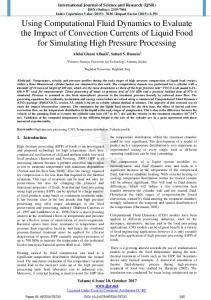
Distance (sphere diameters) Fig. 3. Comparison between the 3-D computational fluid dynamics (CFD) simulations (symbols in C–F) and the potential flow theory (PFT) (solid lines in C–F) for a sphere vibrating above an infinite flat plane wall. The PFT solution consists of a dipole source above the wall and an image dipole source below the wall to satisfy the zero-normal-flow wall boundary condition. The axis of sphere vibration is either parallel (left column) or perpendicular (right column) to the wall. Iso-pressure contours of the instantaneous pressure field are depicted in (A) and (B). Line plots of the instantaneous pressure (C,D) and pressure gradient (E,F) along the wall are shown for three distances (1.8, 3.5 and 8.5 sphere diameters) between the sphere and the wall. U0, velocity amplitude of the sphere vibration; ρ, fluid density; ω=2πf; p1, p2, pressure values along the wall, which are used to calculate the pressure gradients, dp/ds.
THE JOURNAL OF EXPERIMENTAL BIOLOGY
1500 M. A. Rapo and others Analytic solution,
7
A
5
5
4
4
3
3
2
2
1
1 –0.5
0
0
7
7
6
6
5
5
4
4
3
3
2
2
1
1
y/δ
–1
–0.5
0
0
7
7
6
6
5
5
4
4
3
3
2
2
1
1
0
D
–1
–1
0.5
0
0
7
7
6
6
5
5
4
4
3
3
2
2
1
1
0
–1
0.5 u /U ⬁
0
S U ⬁ /δ
7 6
0
C
CFD,
6
0
B
Analytic solution, u /U ⬁ CFD, u /U ⬁
0
0
0.5
1
0
0.5
1
0
0.5
1
|du/dy | U ⬁ /δ
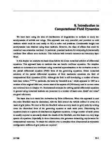
Fig. 4. Comparison between the 3-D computational fluid dynamics (CFD) simulations (symbols) and the analytical solution (solid lines from Eqns 6–8) for the oscillatory boundary layer at the surface of an infinite flat plane wall, created by a sphere vibrating above and parallel to the wall. Vertical (y-) profiles are compared at the wall location directly below the equilibrium position of the sphere. The left column corresponds to the along-wall flow velocity, u, and the right column corresponds to the strain rate, S, and the shear rate, du/dy. A variety of sphere-to-wall distances (r), source vibration magnitudes (U0), frequencies (f), and sphere radii (a) are considered. Four examples are shown here: (A) f=30 Hz, r=10a, U0=0.04 m s–1, phase ωt=0.4π, where ω=2πf and t the time. (B) f=45 Hz, r=20a, U0=0.1 m s–1, phase ωt=1.6π. (C) f=50 Hz, r=3.67a, U0=0.007 m s–1, phase ωt=2π. (D) f=75 Hz, r=40a, U0=0.03 m s–1, phase ωt=2π. δ, Stokes viscous length scale; U⬁, fluid velocity just outside the oscillatory boundary layer.
the 2-D case. The overall pressure field calculated from PFT without the fish body present is different from that obtained from the 3-D CFD simulations but the magnitude of the calculated pressure gradients along the virtual fish mid-plane profile are quite similar to those calculated from the 3-D CFD simulations. This is not the case in the 2-D simulation. The magnitude of the pressure gradient around the fish body is directly related to the location of the dipole source. Spatial variations are most striking when comparing the ipsilateral side of the fish closest with the dipole source and the contralateral side. However, equally noticeable are the differences in magnitude seen between the head and trunk of the fish. In the starting position (Fig. 5B), the magnitude of the pressure gradient is larger on the ipsilateral side near the end of the trunk (blue line) than at the front of the fish (green line). In the second position (Fig. 5C), the magnitude of the pressure gradient is similar for both the head and trunk (green line versus blue and red lines) but a clear difference still exists between the two sides of the fish (blue line versus red line). In the third position (Fig. 5D), the head of the fish is much closer to the dipole source, while the tail is further away. The pressure gradient amplitude has more than quadrupled for the front sections of the head canals (green line). Also, the contrast in pressure gradients between the two sides of the fish has widened (blue line versus red line). Fig. 6 shows the pressure gradients along the lateral line canals of the mottled sculpin (Fig. 2C) based on the 3-D CFD results for the third position of the video sequence (Fig. 5D). Interestingly, the ipsilateral (positive numbers on the horizontal axis) pressuregradient patterns along supraorbital, infraorbital and mandibular canals with different elevations (above and below the eye and along the lower jaw) but largely overlapping azimuths (rostro-caudal extents) tend to converge on the same, nearly redundant pattern. However, patterns on the ipsi- and contralateral side (negative numbers) are dramatically different. Ipsilateral patterns have steeper slopes and distinct zero-crossings (locations where the direction or sign of the pressure gradient changes from positive to negative). In this case, the true source location is near the zero-crossing point on the ipsilateral side. Applying the oscillatory boundary layer solution to real experiments
0
0.5
1
S |du/dy | or U ⬁ /δ U ⬁ /δ
We applied the analytical solutions Eqns 6 and 9 for the oscillatory boundary layer to the results of a number of previous neurophysiological and behavioral experiments designed to measure the threshold sensitivity of SNs in different species and under varying conditions. We used the reported experimental parameters to recompute values of the velocity threshold at the tip of the SN cupula
THE JOURNAL OF EXPERIMENTAL BIOLOGY
CFD of lateral line stimulus and the strain rate threshold at the wall, Swall. The parameters needed for the analysis are a, r, f, U0 and H. The following is a description of the different experiments used in the analysis and the results of the calculations. Kroese et al. (Kroese et al., 1978) used a=1.55 mm oscillating at f=20 Hz parallel to the skin and perpendicular to the longitudinal axis of an SN of the clawed frog (Xenopus laevis), with U0=5⫻10–4 m s–1 and placed at a distance of r=3.75 mm from the skin. They assumed an SN cupula height of 100 μm and found a velocity threshold of 38 μm s–1 based on the potential flow equations. The Stokes viscous length scale for these particular experimental conditions calculated using Eqn 3 is δ=126 μm. Thus, the cupula would be fully immersed in the oscillatory boundary layer flow. From Eqn 6, we find that u at the tip of the cupula after being corrected for the boundary layer effects is 30 μm s–1 (about 21% smaller than Kroese et al.’s threshold estimated from PFT). From Eqn 9, we find that the maximum Swall threshold is 0.45 s–1 and from Eqn 10 the maximum Saverage is 0.30 s–1. Coombs and Janssen estimated velocity thresholds for SNs located along the trunk lateral line of mottled sculpin from neurophysiological measurements (Coombs and Janssen, 1990). The velocity field was produced by an oscillating sphere whose center was placed r=15 mm away from the fish trunk. The radius of the sphere was 3 mm and it was oscillated in a direction perpendicular to the substrate (up/down with respect to the fish) at frequencies in the range 10–500 Hz. The source velocity amplitude of the sphere corresponding to the threshold response, while not explicitly given, can be calculated using the dipole equations (e.g. Pozrikidis, 1997) and the results given in fig. 7 of Coombs and Janssen (Coombs and Janssen, 1990). We estimated that the peak-to-peak acceleration threshold (at the fish) for SNs at 10 Hz is –55 dB re. 1 m s–1 and that the threshold acceleration increases linearly by about 7.5dBoctave–1. From this, we determined that the corresponding source velocity amplitude of the sphere needed to produce the measured peak-topeak acceleration in an unbounded fluid to be about 3.5 mm s–1 for 10 Hz, 5.3 mm s–1 for 50 Hz and 6.3 mm s–1 for 100 Hz. The corresponding velocity amplitude threshold at the tip of the SN cupula based on potential flow equations (with values doubled to account for the presence of the fish body) is 28 μm s–1 at 10 Hz, 42 μm s–1 at 50 Hz and 50 μm s–1 at 100 Hz. The velocity threshold values corrected for the oscillatory boundary layer effects (assuming H=100 μm) are 18 μm s–1 at 10 Hz, 42 μm s–1 at 50 Hz and 54 μm s–1 at 100 Hz, where δ=176 μm at 10 Hz, δ=80 μm at 50 Hz and δ=56 μm at 100 Hz. The velocity threshold for the 10 Hz case is lower than the potential flow case due to the slowing of the flow near the wall, the velocity threshold for the 50 Hz case is unchanged and the velocity threshold for 100 Hz case is actually slightly higher than the potential flow case due to overshoot in the velocity profile (Fig. 7). {At certain distances from the wall the phase lag in viscous stresses is so great that the viscous and pressure terms actually add together. The combination of these forces accelerates the fluid to produce the overshoot [pp. 268–269 in Panton (Panton, 1996)].} The experimental parameter values give maximum Swall of 0.24 s–1 at 10 Hz, 0.78 s–1 at 50 Hz and 1.30 s–1 at 100 Hz. With H=100 μm, the maximum Saverage are 0.18 s–1 at 10 Hz, 0.42 s–1 at 50 Hz and 0.54 s–1 at 100 Hz. Coombs et al. used a vibrating sphere to stimulate CNs and SNs and to see which subsystem was responsible for the orienting response in mottled sculpin (Coombs et al., 2001). When they disabled SNs, the fish was still able to orient towards the vibrating sphere. However, when they disabled CNs, response rates fell to spontaneous levels, indicating that the SNs were not used for
1501
orienting. An alternative explanation is that during the experiment, the stimulus to the SN was below its threshold velocity and strain rate. In their experiments, Coombs et al. used a sphere of radius of 3 mm placed 3–6 cm from the fish (Coombs et al., 2001). The source velocity was 5.5 cm s–1 for the 10 Hz signal and 9.0 cm s–1 for the 50 Hz signal. The maximum velocity at the tip of the cupula [taking viscous effects into account and assuming that H is 100 μm, as in Coombs and Janssen (Coombs and Janssen, 1990)] is 5–36 μm s–1 for 10 Hz (range of values in all cases depend on the distance between the sphere and the fish) and is 11–89 μm s–1 for 50 Hz. The maximum Swall was 0.06–0.47 s–1 for 10 Hz and 0.21–1.66 s–1 for 50 Hz. With H=100 μm, the maximum Saverage are 0.05–0.36 s–1 for 10 Hz and 0.11–0.89 s–1 for 50 Hz. These values are above the SN threshold values measured by Coombs and Janssen (Coombs and Janssen, 1990) when the fish was 3 cm from the sphere but are below threshold values when the fish was 6 cm from the sphere. Alternately, Abdel-Latif et al. showed that blind cave fish could orient toward a vibrating sphere even when the CN subsystem was disabled, indicating that the fish were relying on the SN subsystem to locate the sphere (Abdel-Latif et al., 1990). Their experimental parameters were a=2.5 mm, r=20 cm, f=10–90 Hz and displacement amplitudes = 0.2–1.4 mm. A positive behavioral response for frequencies 50 Hz and 70 Hz was reported for all amplitudes. The corresponding velocity thresholds (taking into account the oscillatory boundary layer effects) based on an SN height of 200 μm (Teyke, 1988) are 0.14–0.96 μm s–1 at 50Hz and 0.19–1.31 μm s–1 at 70 Hz (depending on the displacement amplitude). These values are well below the threshold values of the SNs of other species described above. In addition, the maximum Swall range is 0.0023–0.016 s–1 at 50 Hz and 0.0037–0.026 s–1 at 70 Hz, and the maximum Saverage range is 0.0007–0.048 s–1 at 50 Hz and 0.0010–0.0065 s–1 at 70 Hz. Again these are extremely low values, even acknowledging the possibility of signal startup transients, which from the present numerical simulation briefly increased the maximum wall strain rate up to 4 times the steady state value. DISCUSSION
The results from the 2-D and 3-D simulations are significantly different. Qualitatively, the perturbation to the dipole pressure field due to the presence of fish body is much more prominent in the 2-D CFD results than in the 3-D CFD results. Similarly, the effect of the pectoral fin is also more visible in the 2-D than in the 3-D results. For our specific case, the 2-D and 3-D CFD simulations produced the ‘Mexican-hat’ shaped pressure-gradient patterns with two zero-crossings for the head canal (green line of column 2 in Fig. 5D for 3-D, not shown for 2-D). However, the simulations produced completely different pressure-gradient patterns for the trunk canals (Fig. 5A versus 5B). Quantitatively, the most prominent difference is that the 2-D pressure-gradient magnitudes are 20 times larger than those calculated using the 3-D geometry. Taken together, this raises concerns about using 2-D results to calculate the hydrodynamic stimulus, at least for the present situation of a fish using its lateral line system to locate a vibrating sphere. The 3-D results confirm that it is valid to use PFT to predict the spatial patterns of pressure gradient that affect the canal subsystem. The CFD simulations show that the fish body does perturb the dipole pressure field but only to a small extent, such that the pressure gradients evaluated along the lateral line locations are quite similar to those calculated from the 3-D virtual body case using PFT. This confirms the effectiveness of using PFT to estimate pressure-gradient
THE JOURNAL OF EXPERIMENTAL BIOLOGY
1502 M. A. Rapo and others
Fig. 5. See next page for legend.
THE JOURNAL OF EXPERIMENTAL BIOLOGY
CFD of lateral line stimulus Fig. 5. Comparison between 2-D calculations (A) and 3-D calculations (B), and comparison between 3-D computational fluid dynamics (CFD) (columns 2 and 3 in B–D) and 3-D potential flow theory (PFT, column 4 in B–D) results when the pectoral fins are either included (column 2) or excluded (columns 3 and 4). The calculations correspond to a videorecorded sequence of a mottled sculpin’s step-by-step approach towards an artificial prey – in this case a sinusoidally vibrating sphere [from Coombs and Conley (Coombs and Conley, 1997a)]. The first three steps of the prey-tracking sequence are illustrated, including the initial orienting response at signal onset (A and B are for the same step) followed by two subsequent approach steps (C,D). Each block in columns 2–4 contains a plot of the iso-pressure contours of the normalized instantaneous pressure field that surrounds the sculpin and the vibrating sphere. Plotted in the lower panel are distributions of normalized pressure gradient along the three major portions of the lateral line canal system: the trunk canal on the ipsilateral (I) side of the body with respect to the dipole source (blue curve), the trunk canal on the contralateral (C) side of the body (red curve) and the frontal canals (F) on the head (green curve). T stands for the tail position. The pressure contours in column 4 correspond to the solution of a 3-D (2-D in A) dipole source in an unbounded fluid, unperturbed by the presence of the fish. The pressure gradient values plotted in column 4 are calculated from the unperturbed pressure field but the magnitudes are doubled to account for the potential flow wall-boundary condition of the fish and to facilitate comparison with the CFD solutions. The red arrow in column 2 of A indicates the pressure gradient results for the pectoral fin insertion points. U0, velocity amplitude; ρ, fluid density; ω=2πf; a, sphere radius; dp/ds, pressure gradient; p, pressure.
ρω U 0
dp /ds
patterns to the canal subsystem created by a vibrating sphere in still water (Goulet et al., 2008). The 3-D CFD results do show that the extended fins significantly distort the dipole pressure field locally. The fact that the lateral line trunk canals of the mottled sculpin are routed above the pectoral fins is probably of morphological significance, as it appears that this may limit the distortion in the received signal. Our higher resolved CFD boundary layer simulations using a flatplate model highlight the fact that a vibrating sphere generates an oscillatory boundary layer at the fish’s skin. The resulting flow velocity signal to the SNs and their responses are greatly affected by characteristics of the oscillatory boundary layer, which include its thickness (characterized by the Stokes viscous length scale) and the time-varying and height-varying flow magnitude and direction. Because of the presence of a boundary layer at the fish’s skin, the velocity and velocity gradient patterns that act on the SNs cannot be predicted by PFT. In particular, there is a phase difference (Fig. 4A) between the flow velocity outside and inside the oscillatory boundary layer. Also, there is overshooting of the flow velocity inside the boundary layer (Fig. 4C,D), such that the velocity inside the boundary layer can be greater than the outside flow. Thus, the height of the cupula becomes an important parameter. For example, a cupula with a shorter height that is completely immersed in the
⫻10– 3 1 0.8 0.6 0.4 0.2 0 –0.2 –0.4 –0.6 –0.8 –1 –1 –0.8 –0.6 –0.4 –0.2 0 0.2 0.4 0.6 0.8 1 Tail Contralateral Front Ipsilateral Tail Location along lateral line (BL)
1503
boundary layer will experience a weaker integrated flow over its length than a taller cupula that extends outside the boundary layer. Consequently, a weaker response from the shorter cupula will be expected. Mukai et al. found that the feeding rate of the willow shiner larvae consuming Artemia was proportional to the cupular length on the larva body and saturated at lengths above ~100 μm (Mukai et al., 1994). The trend of their fig. 1 curve relating the feeding rate to the cupular length corresponds well with the trend of the curves shown in Fig. 7 of the present study, which can be interpreted as the maximum tip-to-base velocity difference as a function of neuromast height for three different frequencies. Fig. 7 may provide an explanation to their results, provided that the larvae use the SNs to detect appendage-beating movement of Atemia. There is a minimum cupular displacement that must occur in order for the neuromast to respond, corresponding to a minimum velocity whose drag force causes the displacement. This is called the velocity threshold. Although the velocity threshold may be speciesspecific, the CNs probably respond to internal canal fluid velocities as low as 1–10μms–1 (van Netten, 2006). Inside the subdermal canal, the velocity is driven by the pressure difference between pore openings, which translates to an acceleration threshold of 0.1–1 mm s–2 (van Netten, 2006). The SNs respond to as little as 25–60 μm s–1 (for a review, see van Netten, 2006). These results were obtained using PFT with the assumption that the cupular height is larger than the boundary layer thickness. Using our analytical treatment, we showed that the oscillatory boundary layer formed at the fish’s skin should be taken into account when estimating these velocity thresholds. The oscillatory boundary layer correction can be significant depending on the cupular height relative to the boundary layer thickness. Re-analysis of Coombs and Janssen (Coombs and Janssen, 1990) gives a threshold velocity range of 18–54 μm s–1 over a frequency range of 10–100 Hz, when the oscillatory boundary layer effects are taken into account. The velocity threshold can also be defined as the maximum tip-to-base velocity difference experienced by the cupula, because the base velocity is zero. This is species-specific and depends on a number of parameters, including cupular height and shape, as well as internal cupula stiffness (McHenry et al., 2008). From CFD outputs, one may calculate maximum wall-strain rates, which are a measure of the near-wall fluid-parcel deformation probably experienced by the SNs and are independent of cupular height. For the mottled sculpin of the Coombs et al. (Coombs et al., 2001) experiment, the maximum wall strain rates given in the previous section corresponded to the threshold values of SNs (either just above or just below, depending on the starting distance of the fish from the vibrating dipole source). At the same time, the acceleration experienced by the lateral line canal subsystem (based on Fig. 6) is 5–50 mm s–2, which is many times stronger than the reported acceleration detection thresholds of CNs. This is consistent
Trunk canals Infraorbital canals
Fig. 6. The complete dipole source pressure-gradient signal to the whole canal lateral line system, calculated from 3-D computational fluid dynamics (CFD) and evaluated for strike position No. 3 as shown in Fig. 5D. U0, velocity amplitude; ρ, fluid density; ω=2πf; dp/ds, pressure gradient.
Supraorbital canals Mandibular canals Occipital canal
THE JOURNAL OF EXPERIMENTAL BIOLOGY
1504 M. A. Rapo and others δ
60
Predicted with boundary layer effects included Estimated from potential flow theory
40
uPFT
20
f=10 Hz, U0=3.5 mm s–1, r=15 mm
0 0
100 δ
u (μm s−1)
60
200
300
400
500
600
uPFT
40 20
f=50 Hz, U0=5.3 mm s–1, r=15 mm
0 0 60
Fig. 7. The maximum tip velocity experienced by the superficial neuromasts (SNs) as a function of the neuromast height. The plot was generated analytically based on the experimental conditions used by Coombs and Janssen (Coombs and Janssen, 1990) – sphere radius, r, of 3 mm vibrating in a direction perpendicular to the frontal plane of the fish at frequencies, f, of 10, 50 and 100 Hz and with velocity amplitude, U0, of 3.5 mm s–1, 5.3 mm s–1 and 6.3 mm s–1. The distance from the sphere center to the fish surface was 15 mm. The solid circle is the potential flow result for an SN with cupula height of 100 μm. u, x velocity component.
100
200
300
400
500
600
δ uPFT
40 20 f=100 Hz, U0=6.3 mm s–1, r=15 mm 0 0
100
200 300 400 Superficial neuromast height (μm)
500
with the conclusion that the acceleration-responsive CNs, rather than the velocity-responsive SNs, mediate the mottled sculpin’s orienting behavior to the vibrating sphere (e.g. Coombs et al., 2001). However, all the SN thresholds calculated for the blind cave fish of the AbdelLatif et al. (Abdel-Latif et al., 1990) experiment are extremely low as compared with those numbers obtained for other experiments. This raises concerns regarding claims that the SNs were used for detecting the dipole source, especially since these otophysan fish have pressure-sensitive ears that could have easily detected the pressure changes of a nearby dipole source of the same frequency (Montgomery et al., 2001).
600
ρ φ ω 2-D 3-D
fluid density phase delay 2πf two-dimensional three-dimensional
The authors are grateful to the Woods Hole Oceanographic Institution Academic Programs Office for graduate research support provided to M.A.R. The authors gratefully acknowledge NSF for support of this research under grants IOS0718506 to H.J. and IBN-0114148 to M.A.G. The authors are grateful to two anonymous reviewers, who provided insightful comments that improved the final paper. The authors thank A. H. Techet for helpful discussions.
REFERENCES LIST OF ABBREVIATIONS a C, C1, C2 CFD CN dp/ds du/dy e f H p1, p2 PFT r S S Saverage SN Swall t u u(y,t) U0 U⬁ v w δ Δu μ ν
sphere radius amplitude correction term computational fluid dynamics canal neuromast pressure gradient shear rate mathematical constant e vibration frequency cupula height pressure values at two consecutive nodal points on the profile potential flow theory distance from the sphere to the fish body strain rate tensor strain rate average strain rate superficial neuromast wall strain rate time x velocity component velocity profile velocity amplitude of the sphere vibration fluid velocity just outside the oscillatory boundary layer y velocity component z velocity component Stokes viscous length scale maximum velocity difference between cupular tip and base fluid dynamic viscosity fluid kinematic viscosity
Abdel-Latif, H., Hassan, E. S. and von Campenhausen, C. (1990). Sensory performance of blind Mexican cave fish after destruction of the canal neuromasts. Naturwissenschaften 77, 237-239. Akhtar, I., Mittal, R., Lauder, G. V. and Drucker, E. (2007). Hydrodynamics of a biologically inspired tandem flapping foil configuration. Theor. Comput. Fluid Dyn. 21, 155-170. Anderson, E. J., McGillis, W. R. and Grosenbaugh, M. A. (2001). The boundary layer of swimming fish. J. Exp. Biol. 204, 81-102. Barbier, C. and Humphrey, J. A. C. (2008). Drag force acting on a neuromast in the fish lateral line trunk canal. I. Numerical modelling of external-internal flow coupling. J. R. Soc. Interface (in press). Bleckmann, H. (1993). Role of the lateral line in fish behaviour. In Behaviour of Teleost Fishes, 2nd edn (ed. T. J. Pitcher), pp. 201-246. New York: Chapman & Hall. Bleckmann, H. (2008). Peripheral and central processing of lateral line information. J. Comp. Physiol. A 194, 145-158. Bleckmann, H., Mogdans, J. and Dehnhardt, G. (2001). Lateral line research: the importance of using natural stimuli in studies of sensory systems. In Ecology of Sensing (ed. F. G. Barth and A. Schmid), pp. 149-167. Berlin: Springer-Verlag. Borazjani, I. and Sotiropoulos, F. (2008). Numerical investigation of the hydrodynamics of carangiform swimming in the transitional and inertial flow regimes. J. Exp. Biol. 211, 1541-1558. Carling, J., Williams, T. L. and Bowtell, G. (1998). Self-propelled anguilliform swimming: simultaneous solution of the two-dimensional Navier-Stokes equations and Newton’s laws of motion. J. Exp. Biol. 201, 3143-3166. Cheer, A. Y., Ogami, Y. and Sanderson, S. L. (2001). Computational fluid dynamics in the oral cavity of ram suspension-feeding fishes. J. Theor. Biol. 210, 463-474. Conley, R. A. and Coombs, S. (1998). Dipole source localization by mottled sculpin. III. Orientation after site-specific, unilateral denervation of the lateral line system. J. Comp. Physiol. A 183, 335-344. Coombs, S. (2001). Smart skins: information processing by lateral line flow sensors. Auton. Robots 11, 255-261. Coombs, S. and Conley, R. A. (1997a). Dipole source localization by mottled sculpin. I. Approach strategies. J. Comp. Physiol. A 180, 387-399. Coombs, S. and Conley, R. A. (1997b). Dipole source localization by the mottled sculpin. II. The role of lateral line excitation patterns. J. Comp. Physiol. A 180, 401415.
THE JOURNAL OF EXPERIMENTAL BIOLOGY
CFD of lateral line stimulus Coombs, S. and Janssen, J. (1989). Peripheral processing by the lateral line system of the mottled sculpin (Cottus bairdi). In The Mechanosensory Lateral Line (ed. S. Coombs, P. Görner and H. Münz), pp. 299-319. New York: Springer-Verlag. Coombs, S. and Janssen, J. (1990). Behavioral and neurophysiological assessment of lateral line sensitivity in the mottled sculpin, Cottus bairdi. J. Comp. Physiol. A 167, 557-567. Coombs, S. and Montgomery, J. C. (1999). The enigmatic lateral line system. In Comparative Hearing: Fishes and Amphibians (ed. R. R. Fay and A. N. Popper), pp. 319-362. New York: Springer-Verlag. Coombs, S., Janssen, J. and Webb, W. W. (1988). Diversity of lateral line systems: evolutionary and functional considerations. In Sensory Biology of Aquatic Animals (ed. J. Atema, R. R. Fay, A. N. Popper and W. N. Tavolga), pp. 553-593. New York: Springer-Verlag. Coombs, S., Janssen, J. and Montgomery, J. C. (1992). Functional and evolutionary implications of peripheral diversity in lateral line systems. In The Evolutionary Biology of Hearing (ed. D. B. Webster, R. R. Fay and A. N. Popper), pp. 267-294. New York: Springer-Verlag. Coombs, S., Hastings, M. and Finneran, J. (1996). Modeling and measuring lateral line excitation patterns to changing dipole source locations. J. Comp. Physiol. A 178, 359-371. Coombs, S., Finneran, J. J. and Conley, R. A. (2000). Hydrodynamic image formation by the peripheral lateral line system of the Lake Michigan mottled sculpin, Cottus bairdi. Philos. Trans. R. Soc. Lond. B Biol. Sci. 355, 1111-1114. Coombs, S., Braun, C. B. and Donovan, B. (2001). The orienting response of Lake Michigan mottled sculpin is mediated by canal neuromasts. J. Exp. Biol. 204, 337348. Curcic-Blake, B. and van Netten, S. M. (2006). Source location encoding in the fish lateral line canal. J. Exp. Biol. 209, 1548-1559. Denton, E. J. and Gray, J. A. B. (1983). Mechanical factors in the excitation of clupeid lateral lines. Proc. R. Soc. Lond. B Biol. Sci. 218, 1-26. Denton, E. J. and Gray, J. A. B. (1988). Mechanical factors in the excitation of the lateral lines of fishes. In Sensory Biology of Aquatic Animals (ed. J. Atema, R. R. Fay, A. N. Popper and W. N. Tavolga), pp. 596-617. New York: Springer-Verlag. Dijkgraaf, S. (1963). The functioning and significance of the lateral-line organs. Biol. Rev. 38, 51-105. Goulet, J., Engelmann, J., Chagnaud, B. P., Franosch, J. M. P., Suttner, M. D. and van Hemmen, J. L. (2008). Object localization through the lateral line system of fish: theory and experiment. J. Comp. Physiol. A 194, 1-17. Hassan, E. S. (1985). Mathematical analysis of the stimulus for the lateral line organ. Biol. Cybern. 52, 23-36. Hassan, E. S. (1992a). Mathematical description of the stimuli to the lateral line system of fish derived from a three-dimensional flow field analysis. I. The cases of moving in open water and of gliding towards a plane surface. Biol. Cybern. 66, 443452. Hassan, E. S. (1992b). Mathematical description of the stimuli to the lateral line system of fish derived from a three-dimensional flow field analysis. II. The case of gliding alongside or above a plane surface. Biol. Cybern. 66, 453-461. Hassan, E. S. (1993). Mathematical description of the stimuli to the lateral line system of fish, derived from a three-dimensional flow field analysis. III. The case of an oscillating sphere near the fish. Biol. Cybern. 69, 525-538. Janssen, J. (2004). Lateral line sensory ecology. In The Senses of Fish: Adaptations for the Reception of Natural Stimuli (ed. G. von der Emde, J. Mogdans and B. G. Kapoor), pp. 231-264. New Delhi: Narosa Publishing House. Jiang, H. and Grosenbaugh, M. A. (2006). Numerical simulation of vortex ring formation in the presence of background flow with implications for squid propulsion. Theor. Comput. Fluid Dyn. 20, 103-123.
1505
Jones, W. R. and Janssen, J. (1992). Lateral line development and feeding behavior in the mottled sculpin, Cottus bairdi (Scorpaeniformes: Cottidae). Copeia 1992, 485492. Kalmijn, A. J. (1988). Hydrodynamic and acoustic field detection. In Sensory Biology of Aquatic Animals (ed. J. Atema, R. R. Fay, A. N. Popper and W. N. Tavolga), pp. 83-130. New York: Springer-Verlag. Kalmijn, A. J. (1989). Functional evolution of lateral line and inner ear sensory systems. In The Mechanosensory Lateral Line (ed. S. Coombs, P. Görner and H. Münz), pp. 187-215. New York: Springer-Verlag. Kern, S. and Koumoutsakos, P. (2006). Simulations of optimized anguilliform swimming. J. Exp. Biol. 209, 4841-4857. Kroese, A. B. and Schellart, N. A. M. (1992). Velocity- and acceleration-sensitive units in the trunk lateral line of trout. J. Neurophysiol. 68, 2212-2221. Kroese, A. B. A., Van der Zalm, J. M. and Van den Bercken, J. (1978). Frequency response of the lateral-line organ of Xenopus laevis. Pflügers Arch. 375, 167-175. Liu, H., Wassersug, R. J. and Kawachi, K. (1996). A computational fluid dynamics study of tadpole swimming. J. Exp. Biol. 199, 1245-1260. Liu, H., Wassersug, R. and Kawachi, K. (1997). The three-dimensional hydrodynamics of tadpole locomotion. J. Exp. Biol. 200, 2807-2819. McHenry, M. J., Strother, J. A. and van Netten, S. M. (2008). Mechanical filtering by the boundary layer and fluid-structure interaction in the superficial neuromast of the fish lateral line system. J. Comp. Physiol. A 194, 795-810. Mogdans, J. (2005). Adaptations of the fish lateral line for the analysis of hydrodynamic stimuli. Mar. Ecol. Prog. Ser. 287, 289-292. Montgomery, J. C., Coombs, S. and Halstead, M. (1995). Biology of the mechanosensory lateral line in fishes. Rev. Fish Biol. Fish. 5, 399-416. Montgomery, J. C., Coombs, S. and Baker, C. F. (2001). The mechanosensory lateral line of hypogean fish. Environ. Biol. Fishes 62, 87-96. Mukai, Y. (2006). Role of free neuromasts in larval feeding of willow shiner Gnathopogon elongatus caerulescens Teleostei, Cyprinidae. Fish. Sci. 72, 705-709. Mukai, Y., Yoshikawa, H. and Kobayashi, H. (1994). The relationship between the length of the cupulae of free neuromasts and feeding ability in larvae of the willow shiner Gnathopogon elongatus caerulescens (Teleostei, Cyprinidae). J. Exp. Biol. 197, 399-403. Münz, H. (1985). Single unit activity in the peripheral lateral line system of the cichlid fish Sarotherodon niloticus L. J. Comp. Physiol. A 157, 555-568. Münz, H. (1989). Functional organization of the lateral line periphery. In The Mechanosensory Lateral Line (ed. S. Coombs, P. Görner and H. Münz), pp. 283297. New York: Springer-Verlag. Panton, R. L. (1996). Incompressible Flow, 2nd edn. New York: John Wiley. Pozrikidis, C. (1997). Introduction to Theoretical and Computational Fluid Dynamics. New York: Oxford University Press. Rapo, M. A. (2009). CFD study of hydrodynamic signal perception by fish using the lateral line system. PhD thesis, Massachusetts Institute of Technology/Woods Hole Oceanographic Institution, USA. Schellart, N. A. M. and Wubbels, R. L. (1997). The auditory and mechanosensory lateral line system. In The Physiology of Fishes (ed. D. H. Evans), pp. 283-312. New York: CRC Press. Teyke, T. (1988). Flow field, swimming velocity and boundary layer: parameters which affect the stimulus for the lateral line organ in blind fish. J. Comp. Physiol. A 163, 53-61. van Netten, S. M. (2006). Hydrodynamic detection by cupulae in a lateral line canal: functional relations between physics and physiology. Biol. Cybern. 94, 67-85. Weeg, M. S. and Bass, A. H. (2002). Frequency response properties of lateral line superficial neuromasts in a vocal fish, with evidence for acoustic sensitivity. J. Neurophysiol. 88, 1252-1262.
THE JOURNAL OF EXPERIMENTAL BIOLOGY