Acta Cybernetica 00 (0000) 1–20.
Using Genetic Algorithms in Computer Vision: Registering Images to 3D Surface Model∗ Zsolt Jank´o†, Dmitry Chetverikov† and Anik´o Ek´art‡
Abstract This paper shows a successful application of genetic algorithms in computer vision. We aim at building photorealistic 3D models of real-world objects by adding textural information to the geometry. In this paper we focus on the 2D–3D registration problem: given a 3D geometric model of an object, and optical images of the same object, we need to find the precise alignment of the 2D images to the 3D model. We generalise the photo-consistency approach of Clarkson et al. who assume calibrated cameras, thus only the pose of the object in the world needs to be estimated. Our method extends this approach to the case of uncalibrated cameras, when both intrinsic and extrinsic camera parameters are unknown. We formulate the problem as an optimisation and use a genetic algorithm to find a solution. We use semi-synthetic data to study the effects of different parameter settings on the registration. Additionally, experimental results on real data are presented to demonstrate the efficiency of the method. Keywords: photo-consistency, uncalibrated images, photorealistic models
1
Introduction
Building photorealistic 3D models of real-world objects is a fundamental problem in computer vision and computer graphics. During the last years a number of ambitious projects [4, 17, 25] have been started around the world to digitise cultural heritage objects. Exhibiting 3D models of these objects in a virtual museum provides easy access to them. Furthermore, 3D models of real objects can also be used for surgical simulations in medical imaging, for e-commerce, architecture or entertainment (movies, computer games). ∗ This
work was supported by EU Network of Excellence MUSCLE (FP6-507752) and Automation Research Institute, Budapest, Kende u. 13-17, H-1111 Hungary and E¨ otv¨ os Lor´ and University, Budapest; E-mail: {janko,csetverikov}@sztaki.hu ‡ Aston University, School of Engineering and Applied Science, Computer Science, Aston Triangle, B4 7ET Birmingham, United Kingdom; E-mail:
[email protected] † Computer
1
2
Zsolt Jank´o, Dmitry Chetverikov and Anik´o Ek´ art
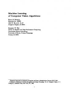
Photorealistic 3D models must have precise geometry as well as detailed texture on the surface. Active and passive methods for creating such models are discussed in [35]. The methods are based on different principles. They use different techniques to reconstruct the object surface, acquire its texture and map the texture onto the surface. The geometry can be measured by various methods of computer vision. When precise measurements are needed, laser scanners are often used. However, most laser scanners do not provide texture and colour information. Even when they do, the data provided are not accurate enough. (See [35] for a detailed discussion.) Whatever the sources of geometric and textural information are, the problem of data fusion, or registration, is to be addressed. In this paper we consider the case when the two sources are independent. We approach the problem of combining precise geometry with high quality images by using genetic algorithms. A number of approaches to the above registration problem have been proposed. In [19] and [20] we introduced a novel method based on photo-consistency. The novelty of our method consists in using uncalibrated cameras—in contrast to Clarkson et al. [8] who need a calibrated setup—and applying a genetic algorithm. Below we describe the problem of photo-consistency based registration and give a summary of our approach. The mathematical formulation of the registration problem is the following. Two input images, I1 and I2 , and a 3D model are given. They represent the same object. (See an example in Figure 1.) The only assumptions about the environment are that the lighting conditions are fixed and the cameras have identical sensitivity1 . All other camera parameters may differ and are unknown. The 3D model consists of a 3D point set P and a set of normal vectors assigned to the points. P is obtained by a hand-held 3D scanner and then triangulated by the robust algorithm of K´ os [22]. This algorithm provides the normal vectors as well.
Images
3D model
Figure 1: Shell dataset. To project the object surface to the image plane, the finite projective camera model [14] is used: u ≃ P X, where u is an image point, P the 3 × 4 projection matrix and X a surface point. (≃ means that the projection is defined up to an unknown scale.) The task of registration is to determine the precise projection matrices, P1 and P2 , for both images. The projection matrix P has 12 elements but only 11 degrees of 1 The
latter can be easily achieved if the images are taken by the same camera.
Registering Images to 3D Surface Model
3
freedom, since it is up to a scale factor. We denote the collection of the 11 unknown parameters by p, which represents the projection matrix P as an 11-dimensional parameter vector. Values of p1 and p2 are sought such that the images are consistent in the sense that the corresponding points—different projections of the same 3D point—have the same colour value. Note that the precise mathematical definition is valid only when the surface is Lambertian, that is, the incoming light is reflected equally to every direction on the surface. This is usually true for diffuse surfaces. Formally, we say that images I1 and I2 are consistent by P1 and P2 (or p1 and p2 ) if for each X ∈ P: u1 = P1 X, u2 = P2 X and I1 (u1 ) = I2 (u2 ). (Here Ii (ui ) is the colour value in point ui of image Ii .) This type of consistency is called photo-consistency [8, 23]. The photo-consistency holds for accurate estimates for p1 and p2 . Inversely, misregistered projection matrices mean much less photo-consistent images. The cost function introduced in [20] is the following: Cφ (p1 , p2 ) =
1 X kI1 (P1 X) − I2 (P2 X)k2 . |P|
(1)
X∈P
Here φ stands for photo-inconsistency while |P| is the number of points in P. Difference of the colour values kI1 − I2 k can be defined by a number of different colour models. (Details are discussed in section 5.1.) Finding the minimum of the cost function (1) over p1 and p2 yields estimates for the projection matrices. In spite of the simplicity of the cost function Cφ (p1 , p2 ), finding the minimum is a difficult task. Due to the 22-dimensional parameter space and the unpredictable shape of Cφ (p1 , p2 ), the standard local nonlinear minimisation techniques failed to provide reliable results. We have tested a number of widely used optimisation methods: Newton-like methods, the Broyden-Fletcher-Goldfarb-Shanno (BFGS) variable metric method and the Levenberg-Marquardt algorithm. Experiments have shown that local search techniques terminate every time in local minima quite far from the expected global optimum. The global nonlinear optimisation technique of Csendes [9] has also been tested. However, the stochastic optimisation method did not yield acceptable results either. The randomness of a stochastic method is excessive, and it does not save nearly good solutions. In contrast, elitist genetic algorithms preserve the most promising results and try to improve them. (Running a GA without elitism yields unstable and imprecise results, similarly to the stochastic optimisation.) The methods mentioned above and other modern techniques, such as simulated annealing and tabu search process one single solution. In addition to performing a local search, simulated annealing and tabu search have specific built-in mechanisms to escape local optima. In contrast, genetic algorithms work on a population of potential solutions, which compete for survival. The competition is what makes GAs essentially different from single solution processing methods [26]. Consequently we decided to apply a genetic algorithm, as a time-honoured global search strategy. Parts of this work have already been presented in papers [19, 20] and [21]. In this study we present the complete method, including a detailed discussion of
4
Zsolt Jank´o, Dmitry Chetverikov and Anik´o Ek´ art
implementation problems, as well as the analysis of the method by systematic tests using different genetic settings and different colour models. The structure of this paper is as follows. In section 2 we give an overview of genetic algorithms and related work on the 2D–3D registration problem. Section 3 presents our registration method based on a genetic algorithm, while section 4 discusses implementation details. In section 5 the method is analysed by tests on semi-synthetic data using different parameter settings. Experimental results on real data are also shown. Finally, section 6 concludes the paper by summarising its contribution.
2 2.1
Overview Genetic Algorithms
To make this study more accessible, we need to devote a section to a brief overview of genetic algorithms, without aiming at completeness. For details the reader is referred to [12] or [2, 3]. Genetic algorithm is a global search technique that imitates natural biological evolution: the algorithm, starting from an initial population of potential solutions and preserving the best individuals, produces new population after new population, obtaining better and better approximations to a solution. At each generation, individuals are selected and bred together, resulting in a new set of approximations. The higher the level of fitness of an individual, the greater its chance of being selected. This fitness-driven selection leads to the evolution of populations of individuals that are better than the populations of their ancestors. In nature individuals are determined by their genes in their chromosomes. In computing genes and chromosomes can be represented by strings: lacing the strings of the genes sequentially gives the string of the chromosome. The most commonly used alphabet of the strings is binary {0,1}, but other alphabets are also used, e.g., integer or real-valued numbers, depending on which is the most suitable for the given problem. Note that further on we shall use the word allele instead of gene, which is a possible variant of the same gene occupying a position (locus) in a chromosome. To improve the population, better individuals should have larger chance to be selected than worse individuals. The goodness of an individual is given by a fitness function. Various selection strategies can be used, those using the fitness values (e.g., roulette wheel selection), or the simple uniform selection, that does not use the level of fitness. Selected individuals are “mated” and new individuals are produced from them, for instance, by interchanging their corresponding alleles. The method of mating is determined by the selected crossover strategy. New individuals can also be created by mutation. The mutation strategy determines how an individual can be mutated. For instance, in Gaussian mutation the value of a selected allele is changed by a random value taken from a Gaussian distribution.
Registering Images to 3D Surface Model
5
The simple GA cannot guarantee the improvement of the population. However, carrying the best individual(s) over to the next generation assures that it will not be worse either. This behaviour of GA is referred to as elitism. It is important to emphasise that GA is non-deterministic: different runs yield different results depending on the seed of the random number generator. However, when the problem does not have one single solution, or when different solutions close to the best one are acceptable, GA is useful and often works better than traditional methods.
2.2
Related Work
Several 2D–3D registration methods exist in computer vision and its medical applications. Most of these methods are based on corresponding feature pairs: features are extracted both from the 3D surface and in the images, and correspondences are searched for. The simplest features are points [10]. Haider and Kaneko [13] look for edges both in 2D and in 3D, and define a 3D edge as a set of 3D surface points which is a 2D edge in the projected space. Stamos et al. [31] localise 2D and 3D lines and search for correspondences. This method has limited applicability, but can be useful when the objects are buildings with many line features. Ikeuchi et al. [17] also use lines and edges to calibrate cameras. The disadvantages of featurebased methods are that features are often difficult to localise precisely in 3D and, in addition, defining a similarity function between 2D and 3D features is not easy. Another approach is to use the contour or the shape of the object to match to its projection. Hern´ andez [16] defines a silhouette coherence criterion, but he does not use the 3D model of the object. 3D reconstruction from silhouettes and camera calibration are accomplished simultaneously. Such methods are more precise than feature-based methods, but in case of symmetric objects they are completely useless. Intensity-based techniques can also be applied to align the images to the 3D model. In order to find correspondences, colour information of image pixels can be used as well as constraints on the gradient. The method of Umeda et al. [32] is based on range intensity images. They use a special range sensor that measures the property of the reflected light. The amount of the reflected light is related to the reflectance ratio of the measured point, thus the obtained image describes the reflectance of the object. This image is referred to as range intensity image. Colour images taken by a camera are registered to the range images by using constraints on the gradients of the colour images and of the range intensity images. Viola et al. [33] search for the alignment of a 3D model and an optical image by maximising their mutual information. They use a geometric transformation that maps model points to image points, and also use an imaging function describing lighting conditions, surface properties, and imaging device characteristics. The registration problem can then be formulated as maximising the mutual information between the optical image intensities and the surface normal vectors of the model. Leventon et al. [24] and Clarkson et al. [8] have shown that a registration algorithm based on maximising the mutual information can be improved by using multiple rather than single images. The algorithm in [8] applies photo-consistency
6
Zsolt Jank´o, Dmitry Chetverikov and Anik´o Ek´ art
to find precise registration of 2D optical images of a human face to a 3D surface model. It uses calibrated images, thus the problem is reduced to estimating the pose of the cameras. Our method generalises this approach to the case of uncalibrated cameras, when both intrinsic and extrinsic parameters are unknown. Genetic Algorithms in Registration Methods None of the methods mentioned above use genetic algorithms, since the optimisation problems they consider are easier and are solved faster by conventional non-linear iterative strategies. In our case the size of the parameter space and the complexity of the cost function motivated the use of genetic algorithm-based optimisation. While the application of genetic algorithms in 2D–3D registration methods has not been significant so far, several methods use evolutionary techniques to register 3D data or range images. In [29] Renner and Ek´ art provide a summary of genetic algorithms in computer aided design. Jacq and Roux [18] use GAs for registration of 3D medical images. GAs are also used to register 3D surfaces [5] as well as range images [7]. In contrast to the 2D–3D registration, numerous methods exist to precisely register 3D data by iterative algorithms like the Iterative Closest Point and its variants [6]. Here, the task of GA-based methods is usually to automatically provide rough pre-registration of the surfaces needed by the iterative methods as an initial state close to the solution.
3
Genetic Algorithm-Based Optimisation
In section 1 we have formulated the registration problem and introduced the cost function. In this section the optimisation method is described. Incorporating domain knowledge always makes GAs more effective. To narrow the search domain and accelerate the method, it is worth starting the search from a good initial state. We decided to pre-register the images and the 3D model manually, since this operation is simple and fast compared to the 3D scanning, which is also done manually. Our assumption was that the photo-consistency based registration would make the result more accurate. The tests justify this assumption. Figure 2 summarises the proposed two-step method. The manual preregistration provides the rough estimates P10 and P20 of the projection matrices P1 and P2 , respectively. Then P10 and P20 are refined by minimising the photoconsistency based cost function (1) by a genetic algorithm. Note that each image is pre-registered to the 3D model separately, while the final precise registration involves simultaneous registration of both images to the model. Designing the genetic algorithm for a given problem needs careful consideration. For general practical advice, the reader is referred to [26]. We use fixed-length vectors of bounded real numbers as representation. The individuals of the population are chosen from the neighbourhood of the parameter vector obtained by the manual pre-registration. The individual that encodes the pre-registered parameter vector is inserted in the initial population to avoid losing it. The values of the genes of the
7
Registering Images to 3D Surface Model
Reg 1 image 1
Reg 2 image 2
3D model manual pre−registration P10
image 1
P20 3D model
image 2
photo−consistency based registration
P1 , P2
Figure 2: Block-diagram of proposed method.
remaining individuals are from the intervals defined by the pre-registered values plus a margin of ±ǫ. In our experiments ǫ was set to values between 1% and 3%, depending on the meaning and the importance of the corresponding parameter. For instance, small changes in parameter principal point can yield great deformations in projection, hence the interval of this parameter is set to ±0.5%, in contrast to the focal length, where the interval is ±2%. Details of camera parameters will be discussed in section 4.2. During the initialisation the individuals are pre-selected: the useless individuals for which the cost function yields an extreme value are omitted. This prevents the genetic algorithm from jumping around the search space; since the aim of the method is to refine the initial state, small changes in the values are sufficient. Nevertheless, we tested the method without this restriction, as well, but the convergence was slower and the results were worse. To avoid premature convergence we decided to run the algorithm three times: the algorithm starts three times from the beginning, preserving only the best individual from the previous step and re-initialising the whole population. An iteration is finished if Ng generations have been created, or if the best of the population has changed 10 times. (The setting of Ng is discussed later, in section 5.1.) Our genetic algorithm is shown in Algorithm 1.
4
Implementation Details
We have chosen the GAlib package [34] written by Matthew Wall at the MIT, to implement our genetic algorithm-based method. For tests we mainly used the following parameter settings of GA as default: Steady state algorithm, Tournament
8
Zsolt Jank´o, Dmitry Chetverikov and Anik´o Ek´ art
Algorithm 1 Genetic algorithm. 1: BEST ←− manual pre-registration. 2: for i = 1, . . . , 3 do 3: Generate initial population around BEST. 4: BEST ←− best of the population. 5: repeat 6: Calculate cost function values. 7: Apply genetic operators, create new population. 8: BEST ←− best of the population. 9: until (Ng generations created) or (BEST changed 10 times) 10: end for
selector, Swap mutation, Uniform crossover, 250 individuals in the population, mutation probability 0.1 and crossover probability 0.7.
4.1
Robustness
In registration and correspondence, robustness is a critical issue. Minimising the cost function (1) is a least-squares method, therefore it is not robust, due to the inconsistencies produced by outliers, typically, by occluded points. In [8], the visibility is checked by ray tracing, but here we use surface normals for this purpose. Our implementation is less accurate but much faster, which is more important in this case. The essence of our algorithm is to discard the point when the scalar product of the normal vector and the unit vector pointing towards the camera falls below a threshold. The product is the cosine of the angle between the two vectors. Typically, the threshold is set at 0.5, which discards some mutually visible points, but still leaves enough points for reliable registration. In computer vision this method is usually referred to as backface culling. Backface culling works well when the surface is convex but fails when it is concave. The 3D models we use at registration are reduced to contain only 1000–1500 points, which is usually enough to obtain good result. It means that in most cases the input 3D models are rough and smooth, and they are nearly convex. However, it is clear that the trivial method for checking visibility cannot guarantee that all invisible points will be filtered out. The remaining false points are considered as outliers, as well as the false inconsistencies caused by texture periodicity or the object boundary. To suppress the remaining outliers, the cost function (1) was modified in a robust manner. Two variants of modification were considered: the Trimmed Squares (TS) and the α-trimmed mean [28]. Both techniques have a single parameter, α. In TS, α is the rate of the largest squares which are discarded. In the α-trimmed mean, both smallest and largest values are rejected: when α is close to 0.5, the median is used. In our experiments, we used α = 0.2. In attempts to improve the method, we have tested a few other cost functions. However, the variance of the colour values [8] or the Modified Normalised Cross
Registering Images to 3D Surface Model
9
Correlation [30] yielded worse results than the robust least-squares described above. The sizes of our test images are 512 × 512 or 1024 × 1024. It seemed reasonable to reduce the size and apply image pyramids for the registration, but the results did not improve significantly.
4.2
Constraints on the Camera Model
As already mentioned, our original method applied optimisation in the full 22dimensional parameter space. The size of the space and the non-smoothness of the cost function are two critical problems that make the search difficult and timeconsuming despite the restrictions due to the manual pre-registration. To improve the efficiency of the optimisation process, we impose some reasonable constraints on the camera model, as suggested in [14]. Note that using the finite projective camera model without camera distortion is already a constraint which works well in practice. The projection matrix can be decomposed as P = K [R | −R t], where K is the 3 × 3 camera calibration matrix and the 3 × 3 rotation matrix R describes the orientation, the 3-dimensional translation vector t the location of the camera. The camera calibration matrix can be expressed in form αu s −u0 αv −v0 . K= (2) 1 Here αu and αv represent the focal length of the camera in terms of pixel dimensions in the u and v directions of the image plane, respectively, s is the skew parameter and (u0 , v0 ) is the so-called principal point. For most cameras the skew parameter is zero. It is also usual to assume that the pixels are squared, that is the ratio of αu and αv is equal to 1. Thus the camera calibration matrix can be simplified to the so-called pinhole camera model : f −u0 f −v0 , (3) K= 1 with focal length f . These simplifications reduce the number of the degrees of freedom from 22 to 18. Although the decrease is not large, in this case every reasonable reduction is important. Therefore we also applied a commonly used assumption, that the principal point is close to the image centre. This assumption does not reduce the number of the parameters, but the search space becomes more restricted. In the previous sections we did not specify the ǫ values for the intervals of the genes. Considering the simplifications detailed above, the values we use are the following: • focal length: ±2% • principal point: ±0.5%
10
Zsolt Jank´o, Dmitry Chetverikov and Anik´o Ek´ art
• camera translation: ±3% • camera rotation: ±1◦ .
5 5.1
Experiments Quantitative Assessment on Semi-Synthetic Data
To quantitatively assess the results, the algorithm was run on semi-synthetic data with ground truth. We obtain these data by covering the triangular mesh of the original Shell, Frog and Bear datasets (see Figures 3, 4 and 5) with different textures. The textures were obtained from the photos of the original objects. Two views of these objects produced by a visualisation program provide the input images for which the projection matrices are completely known. The projection error is measured as follows: the 3D point set P is projected onto the image planes by both the ground truth and the estimated projection matrices, and then the average distance between the corresponding image points is calculated. Formally, if PiG are the ground truth, Pi the estimated projection matrices, then E(P1 , P2 ) =
1 X 1 X
P G X − Pi X . i 2 i=1,2 |P|
(4)
X∈P
By this metric the average error of the manual pre-registration is 18–20 pixels for the Shell and 12–15 pixels for the Bear and the Frog. Tables 1–8 show the results of the method executed with different settings. In each case 10 runs were performed and the mean and the confidence interval were calculated. Next we show the influence of different colour models and different genetic settings on the registration. Colour Models An important question in the case of methods which compare colours is how to calculate colour differences, which colour model provides the best result. We have tested four different models: RGB, XYZ, CIE LAB and CIE LUV. Each model consists of three components, and colour differences were calculated as the simple sum of squared differences in the three components. Table 1 shows the results for the Shell, the Bear and the Frog datasets. In the literature CIE LUV and CIE LAB are usually used to compare colours, since the perception of colour difference in RGB and XYZ is highly non-uniform. Indeed, our tests have shown that uniform models perform slightly better, but the difference in projection error is not significant. In our experimental data the illumination changes are small. Tests were run both on diffuse and specular data. As it is expected, the error of specular data is significantly greater than that of the diffuse data. This is obvious, since photo-consistency supposes Lambertian reflection. However, one can see
11
Registering Images to 3D Surface Model
that specular errors do not grow extremely and remain below a reasonable limit, due to the robustness of the method and the application of geometric constraints discussed above. If the initial model is relatively good, and consequently geometric constraints are correct, then registration of a specular dataset is fairly good, see the Frog in table 1. Table 1: Projection error using different colour models. Col. model RGB XYZ CIE LAB CIE LUV
Shell Diffuse Specular 7.3 ± 0.4 8.8 ± 0.7 6.7 ± 0.5 11.4±2.2 6.9 ± 0.2 8.9 ± 1.3 6.9 ± 0.5 8.9 ± 1.0
Bear Diffuse Specular 7.8 ± 0.5 9.6 ± 0.2 7.8 ± 0.6 9.3 ± 0.2 6.5 ± 0.5 10.0±0.6 6.7 ± 0.5 9.8 ± 0.5
Frog Diffuse Specular 4.6 ± 0.3 5.9 ± 0.4 4.9 ± 0.3 5.7 ± 0.6 5.2 ± 0.4 6.0 ± 0.3 4.4 ± 0.2 5.7 ± 0.4
Genetic Settings A number of tests have been carried out to check the effects of different genetic settings on the registration. First, we tried two different algorithms: the simple GA of Goldberg [12] and the steady state GA. In the simple GA, we use non-overlapping populations: in each generation an entirely new population is created by crossover and mutation. We also use elitism: the best individual is carried over to the next generation. Elitism is set during all the tests in order to avoid losing good results. The steady state algorithm is similar to the one described by De Jong [11]. Here, we use overlapping populations with an overlap of 25%. Each generation a temporary population of individuals is created and added to the previous population. Then the worst individuals are removed to reduce the population to its original size. The results shown in table 2 are not surprising: the steady state algorithm performs better than the simple GA. The difference in speed can be explained by the termination criterion of the algorithm. As we mentioned above, each iteration terminates if Ng generations were created or if the best individual of the population changed 10 times. The steady state algorithm preserves a number of the best individuals of the population, hence it can create better new individuals than the simple GA, which preserves only the very best individual. Our tests have shown that in the case of the steady state algorithm the best individual changed every 4–5 generations, while in the case of the simple GA this number was 10–15. Therefore, the steady state algorithm terminates much sooner, after fewer iterations. In the next test three different selectors were tried: roulette wheel selector, tournament selector and uniform selector (table 3). Roulette wheel selector picks an individual based on its fitness score relative to the rest of the population. The higher the score, the more likely an individual will be selected. Tournament selector uses the roulette wheel method to choose two individuals, then picks the
12
Zsolt Jank´o, Dmitry Chetverikov and Anik´o Ek´ art
Table 2: Results of different genetic algorithms. Algorithm Simple Steady State
Projection error Shell Bear Frog 7.4 ± 1.0 6.7 ± 0.4 8.9 ± 1.0 6.3 ± 0.8 5.1 ± 0.3 6.6 ± 0.5
Shell 11.1 ± 0.2 6.4 ± 0.3
Time (min) Bear Frog 7.8 ± 0.3 9.9 ± 0.2 4.5 ± 0.3 4.7 ± 0.4
one with the higher score. Uniform selector selects each individual with uniform probability. According to our tests, the non-uniform selectors are slightly better than the uniform selector; however, the difference is not significant. Table 3: Results for different selectors. Selector Roul.wheel Tournament Uniform
Projection error Shell Bear Frog 6.0 ± 0.7 5.1 ± 0.4 6.6 ± 0.8 6.0 ± 0.5 4.6 ± 0.1 6.1 ± 0.8 6.7 ± 0.7 4.9 ± 0.4 7.1 ± 0.6
Shell 6.4 ± 0.3 6.3 ± 0.3 6.6 ± 0.3
Time (min) Bear Frog 4.6 ± 0.3 4.8 ± 0.3 4.5 ± 0.3 4.3 ± 0.3 4.6 ± 0.3 5.0 ± 0.3
Next we have tested a number of different types of mutation and crossover. Here we give only a short description of the operators; for details the reader is referred to [15]. In Gaussian mutation the value of the selected allele is changed by a random value taken from a Gaussian distribution (and then adjusted to the range). Flip mutation gives a random value to a randomly chosen allele, considering bounds. Swap mutation picks two alleles at random and exchanges their values. In uniform crossover the value of each allele of the offspring is randomly chosen from the same alleles of the parents. Even-odd crossover considers two operators: for even crossover, the even alleles of the offspring are taken from one parent and the odd alleles from the other parent. For odd crossover, the opposite is done. In onepoint crossover the two parents’ codes are cut at a randomly chosen position and the end-parts of the parents are exchanged to produce two offspring. In two-point crossover two crossover points are selected at random and the middle part of the parents’ code is exchanged. In partial-match crossover a random position is picked. Let us suppose the values in this position in the two parents are x and y. Then x and y are interchanged throughout both parents’ code. The operation is repeated several times. In order crossover about half of the elements of the offspring are picked from one parent, keeping the order, and the rest from the other parent, also keeping the order. Blend crossover chooses a new value for the offspring allele in the neighbourhood of parent values. Suppose x < y, then the value for the offspring is uniformly chosen from the interval [x − α(y − x), x + α(y − x)]. Arithmetic crossover creates an offspring “between” the two parents. If x and y are the parental allele values, the offspring
13
Registering Images to 3D Surface Model
will become z = x + (1 − α)y where α ∈ [0, 1]. Table 4 shows that different mutations yield very similar error. Flip mutation is slightly better, swap mutation is slightly faster than the others. In the case of the crossovers (table 5), blend and arithmetic crossovers perform better than the others. Table 4: Results for different types of mutation. Mutation Gaussian Flip Swap
Projection error Shell Bear Frog 6.4 ± 0.5 4.7 ± 0.3 5.9 ± 0.6 6.0 ± 0.7 4.7 ± 0.2 5.7 ± 0.5 6.0 ± 0.6 5.0 ± 0.3 6.4 ± 0.8
Shell 9.8 ± 0.3 9.5 ± 0.4 6.4 ± 0.3
Time (min) Bear Frog 6.2 ± 0.4 6.1 ± 0.3 6.2 ± 0.5 6.6 ± 0.6 4.3 ± 0.3 4.3 ± 0.3
Table 5: Results for different types of crossover. Crossover Uniform Even-Odd One-Point Two-Point Partial-match Order Blend Arithmetic
Projection error Shell Bear Frog 6.1 ± 0.7 5.4 ± 0.8 6.6 ± 0.9 6.4 ± 1.0 5.6 ± 0.7 7.3 ± 1.3 6.7 ± 0.8 5.5 ± 0.9 7.0 ± 1.3 6.7 ± 1.2 5.4 ± 0.4 6.6 ± 0.5 8.7 ± 0.8 7.1 ± 1.2 10.0 ± 2.7 8.2 ± 1.0 6.8 ± 0.8 10.5 ± 1.7 6.1 ± 0.9 4.9 ± 0.4 6.0 ± 0.6 5.0 ± 0.5 5.5 ± 0.8 4.9 ± 0.4
Shell 6.4 ± 0.4 6.2 ± 0.4 6.6 ± 0.4 6.5 ± 0.5 3.0 ± 0.1 3.3 ± 0.4 6.4 ± 0.4 6.3 ± 0.4
Time (min) Bear 4.5 ± 0.5 4.5 ± 0.5 4.8 ± 0.4 4.8 ± 0.4 3.4 ± 0.4 3.1 ± 0.3 4.6 ± 0.6 4.6 ± 0.4
Frog 4.4 ± 0.6 4.7 ± 0.4 4.9 ± 0.6 4.5 ± 0.5 4.0 ± 0.1 3.1 ± 0.3 4.3 ± 0.4 4.0 ± 0.4
Table 6 is self-evident. Increasing the population size improves the result and makes the method slower. The difference in error between populations with 250 or 500 individuals is insignificant, hence setting the size of the population to a vicinity of 250 is reasonable. On the other hand, convergence is reached somewhere between 100 and 200 generations, so the results do not significantly depend on whether Ng is set to 100 or 200. Therefore we used 100 generations. Table 6: Results for different population sizes. Pop.size 100 250 500
Projection error Shell Bear Frog 6.8 ± 0.8 6.6 ± 0.8 8.2 ± 1.5 6.0 ± 0.5 4.9 ± 0.4 6.1 ± 0.4 5.8 ± 0.4 4.6 ± 0.1 6.2 ± 0.5
Shell 2.5 ± 0.3 6.5 ± 0.5 12.2 ± 0.5
Time (min) Bear Frog 1.8 ± 0.3 1.8 ± 0.3 4.4 ± 0.3 4.2 ± 0.3 9.2 ± 0.3 8.5 ± 0.6
14
Zsolt Jank´o, Dmitry Chetverikov and Anik´o Ek´ art
The results of tables 7 and 8 are also expected. More frequent mutation increases the randomness, hereby the error and the duration as well. Having the crossover probability 0.9 or 0.7 yields almost the same error, however in the case of 0.7 the method is slightly faster. Table 7: Results for different mutation probabilities. Mut.prob. 0.1 0.3 0.5
Projection error Shell Bear Frog 6.0 ± 0.5 4.7 ± 0.2 5.9 ± 0.9 9.9 ± 2.1 7.1 ± 0.9 9.6 ± 1.4 9.2 ± 1.9 7.5 ± 1.0 10.4 ± 1.1
Shell 6.3 ± 0.3 2.8 ± 0.3 2.0 ± 0.1
Time (min) Bear Frog 4.7 ± 0.3 4.2 ± 0.3 2.9 ± 0.2 3.2 ± 0.3 2.2 ± 0.3 2.7 ± 0.4
Table 8: Results for different crossover probabilities. Cross.prob. 0.9 0.7 0.5
Projection error Shell Bear Frog 5.8 ± 0.6 4.6 ± 0.2 5.8 ± 0.4 5.9 ± 0.6 5.1 ± 0.3 6.3 ± 0.6 6.4 ± 1.0 5.3 ± 0.5 7.4 ± 0.6
Shell 6.4 ± 0.3 5.4 ± 0.3 4.6 ± 0.3
Time (min) Bear Frog 4.9 ± 0.2 5.2 ± 0.3 4.5 ± 0.3 4.6 ± 0.3 3.9 ± 0.2 4.0 ± 0.4
Based on these tests we can conclude that one reasonable setting is as follows: Steady state algorithm with Tournament selector, Flip mutation and Arithmetic crossover, with 250 individuals in the population, mutation probability 0.1 and crossover probability 0.7.
5.2
Results for Real Data
To test the efficiency of the method we also applied it to real data. A number of different datasets were used. Figures 3–7 show the Shell, the Frog, the Bear, the Cat and the Head datasets as well as the textured 3D models obtained. The Shell dataset is interesting because of the periodicity in shape and texture. The Frog and the Head are challenging as their textures are less visible and less characteristic. The Bear and the Cat have both characteristic shape and texture. All 3D models were acquired in our laboratory using the ModelMaker [1] laser scanner, and the images were captured by a digital camera. The 3D models contain tens of thousands of points, but for registration the set was reduced to 1000–1500 points. We used the algorithm of K´os [22] for this just as for triangulation. The dimensions of the images are 512 × 512 or 1024 × 1024. The precision of the registration can be best judged by looking at the stripes of the Shell, as well as the mouth, the eyes, the hand and the feet of the Bear and the Cat. In the case of the Shell both the shape and the texture are periodic, hence
15
Registering Images to 3D Surface Model
Images
3D model
Textured model
Figure 3: Shell dataset and result of registration.
Images
3D model
Textured model
Figure 4: Frog dataset and result of registration.
Images
3D model
Textured model
Figure 5: Bear dataset and result of registration.
precise registration is crucial for photorealism. One can see that the stripes of the texture are in the appropriate position.
16
Zsolt Jank´o, Dmitry Chetverikov and Anik´o Ek´ art
Images
3D model
Textured model
Figure 6: Cat dataset and result of registration.
Images
3D model
Textured model
Figure 7: Head dataset and result of registration.
6
Conclusion
In this paper we have presented a method for registering a pair of high-quality images to a 3D surface model using a genetic algorithm. The registration is performed by minimising a photo-consistency based cost function. The application of the genetic algorithm is reasonable, since the shape of the cost function is rough and unpredictable, with multiple minima. The results of previously studied standard local and global optimisation methods were not acceptable. The aim of this study was to present the complete method in details. Besides the description of the optimisation method and the discussion of implementation details, a number of tests have been carried out to check the effects of different colour models and different genetic parameter settings on the registration. Different settings can lead to significantly different results. The tests were run on three different objects, by which we mean both different geometry and different textures. Results show strong analogy, verifying the general validity of the effects of parameter settings on the method. The tests have shown that by choosing the best settings the projection error of the registration can be decreased from 18–20 pixels, which
17
Registering Images to 3D Surface Model
is the average error of the manual pre-registration, to 5–6 pixels for diffuse and to 8–10 pixels for specular surfaces. Figure 8 visualises the difference between the manual pre-registration and the photo-consistency based genetic registration. The quality of registration in the areas of the mouth, the eyes and the ears is visibly better after the genetic algorithm has been applied. Here again the difference is essential for photorealism.
Manual
Genetic
Figure 8: Difference between manual pre-registration and genetic registration.
Choosing the best parameters for a particular problem requires a lot of experimentation or some sophisticated method. Studies on parameter control in GAs mostly consider controlling one aspect of the algorithm at a time and they use some form of self-adaptation. Michalewicz and Fogel [26] provide a detailed discussion on tuning the algorithm to the problem. Furthermore, there exist metamodelling techniques like the Response Surface Methodology (RSM) [27] to try out parameters in a systematic way. RSM uses quantitative data to describe how the parameters affect the response, to determine the interrelationships among the parameters and to describe the combined effect of all the parameters on the response. However, controlling multiple parameters simultaneously is a current research topic in GAs and is beyond the scope of this paper.
18
Zsolt Jank´o, Dmitry Chetverikov and Anik´o Ek´ art
References [1] 3D Scanners. Modelmaker. URL: http://www.3dscanners.com/. [2] Beasley, David, Bull, David R., and Martin, Ralph R. An overview of genetic algorithms: Part 1, fundamentals. University Computing, 15(2):58–69, 1993. [3] Beasley, David, Bull, David R., and Martin, Ralph R. An overview of genetic algorithms: Part 2, research topics. University Computing, 15(4):170–181, 1993. [4] Bernardini, Fausto, Martin, Ioana M., and Rushmeier, Holly. High-quality texture reconstruction from multiple scans. IEEE Transactions on Visualization and Computer Graphics, 07(4):318–332, 2001. [5] Brunnstr¨ om, K. and Stoddart, AJ. Genetic algorithms for free-form surface matching. In Proc. 13th International Conference on Pattern Recognition, volume 4, pages 689–693, 1996. [6] Chetverikov, Dmitry, Stepanov, Dmitry, and Krsek, Pavel. Robust euclidean alignment of 3D point sets: the trimmed iterative closest point algorithm. Image and Vision Computing, 23(3):299–309, 2005. [7] Chow, Chi Kin, Tsui, Hung Tat, and Lee, Tong. Surface registration using a dynamic genetic algorithm. Pattern Recognition, 37:105–117, 2004. [8] Clarkson, Matthew J., Rueckert, Daniel, Hill, Derek L.G., and Hawkes, David J. Using photo-consistency to register 2D optical images of the human face to a 3D surface model. IEEE Transactions on Pattern Analysis and Machine Intelligence, 23:1266–1280, 2001. [9] Csendes, T. Nonlinear parameter estimation by global optimization – Efficiency and Reliability. Acta Cybernetica, 8:361–370, 1988. [10] David, Philip, DeMenthon, Daniel, Duraiswami, Ramani, and Samet, Hanan. SoftPOSIT: Simultaneous pose and correspondence determination. In Proc. 7th European Conference on Computer Vision, pages 698–714, 2002. [11] De Jong, Kenneth Alan. An analysis of the behavior of a class of genetic adaptive systems. PhD thesis, University of Michigan, 1975. [12] Goldberg, David E. Genetic Algorithms in Search, Optimization, and Machine Learning. Addison-Wesley, 1989. [13] Haider, Ali Md. and Kaneko, Toyohisa. Automated 3D–2D projective registration of human facial images using edge features. International Journal of Pattern Recognition and Artificial Intelligence, 15(8):1263–1276, 2001. [14] Hartley, R. and Zisserman, A. Multiple View Geometry in Computer Vision. Cambridge University Press, 2000.
Registering Images to 3D Surface Model
19
[15] Haupt, Randy L. and Haupt, Sue Ellen. Practical Genetic Algorithms. WileyInterscience, 2004. [16] Hern´ andez, Carlos. Stereo and Silhouette Fusion for 3D Object Modeling from Uncalibrated Images Under Circular Motion. PhD thesis, Ecole Nationale Sup´erieure des T´el´ecommunications, 2004. [17] Ikeuchi, Katsushi, Nakazawa, Atsushi, Hasegawa, Kazuhide, and Ohishi, Takeshi. The great Buddha project: Modeling cultural heritage for VR systems through observation. In Proc. IEEE ISMAR03, 2003. [18] Jacq, JJ. and Roux, C. Registration of 3D images by genetic optimization. Pattern Recognition Letters, 16:823–841, 1995. [19] Jank´ o, Zsolt and Chetverikov, Dmitry. Photo-consistency based registration of an uncalibrated image pair to a 3D surface model using genetic algorithm. In Proc. 2nd International Symposium on 3D Data Processing, Visualization & Transmission, pages 616–622, 2004. [20] Jank´ o, Zsolt and Chetverikov, Dmitry. Registration of an uncalibrated image pair to a 3D surface model. In Proc. 17th International Conference on Pattern Recognition, volume 2, pages 208–211, 2004. [21] Jank´ o, Zsolt, Chetverikov, Dmitry, and Ek´ art, Anik´ o. Using a genetic algorithm to register an uncalibrated image pair to a 3D surface model. International Journal of Engineering Applications of Artificial Intelligence, 19:269– 276, 2006. [22] K´ os, G´eza. An algorithm to triangulate surfaces in 3D using unorganised point clouds. Computing Suppl., 14:219–232, 2001. [23] Kutulakos, K.N. and Seitz, S.M. A Theory of Shape by Space Carving. Prentice Hall, 1993. [24] Leventon, M.E., Wells III, W.M., and Grimson, W.E.L. Multiple view 2D-3D mutual information registration. In Proc. Image Understanding Workshop, 1997. [25] M. Levoy et al. The digital Michelangelo project. ACM Computer Graphics Proceedings, SIGGRAPH, pages 131–144, 2000. [26] Michalewicz, Zbigniew and Fogel, David B. How to Solve It: Modern Heuristics. Springer, 2002. [27] Myers, Raymond H. and Montgomery, Douglas C. Response Surface Methodology. John Wiley & Sons, Inc., 1995. [28] Pitas, I. Digital Image Processing Algorithms. Prentice Hall, 1993.
20
Zsolt Jank´o, Dmitry Chetverikov and Anik´o Ek´ art
[29] Renner, G´ abor and Ek´ art, Anik´o. Genetic algorithms in computer aided design. Computer Aided Design, 35:709–726, 2003. [30] Sara, Radim. Finding the largest unambiguous component of stereo matching. In Proc. 7th European Conference on Computer Vision, volume 2, pages 900– 914, 2002. [31] Stamos, Ioannis and Allen, Peter K. Geometry and texture recovery of scenes of large scale. Computer Vision and Image Understanding, 88(2):94–118, 2002. [32] Umeda, Kazunori, Godin, Guy, and Rioux, Marc. Registration of range and color images using gradient constraints and range intensity images. In Proc. 17th International Conference on Pattern Recognition, volume 3, pages 12–15, 2004. [33] Viola, Paul and Wells III, William M. Alignment by maximization of mutual information. International Journal of Computer Vision, 24(2):137–154, 1997. [34] Matthew Wall. The GAlib genetic algorithm package. URL: http://lancet.mit.edu/ga, 2003. [35] Yemez, Y. and Schmitt, F. 3D reconstruction of real objects with high resolution shape and texture. Image and Vision Computing, 22:1137–1153, 2004. Received ...