MIC2003: The Fifth Metaheuristics International Conference
??-1
Using Simulated Annealing to study behaviour of various Exam Timetabling data sets Edmund Burke∗
Adam Eckersley∗ Barry McCollum† Rong Qu∗
Sanja Petrovic∗
∗ School
of Computer Science & Information Technology University of Nottingham, Nottingham, NG8 1BB, UK {ekb,aje,sxp,rxq}@cs.nott.ac.uk † Queens
University of Belfast Belfast, Northern Ireland
[email protected]
1
Introduction
In this paper we use a simple simulated annealing (SA) metaheuristic as the basis for comparing behaviour of a number of different examination timetabling problems when optimised from initial solutions given by a largest degree graph-colouring heuristic with backtracking. The ultimate aim of our work is to develop a measure of similarity between exam timetabling problems. By similarity we mean that two similar problems will be solved equally well and produce results of an acceptable quality using the same meta-heuristic. To help achieve this we are analysing a group of benchmark data sets, all of which have been optimised using SA. We have also developed a Tabu Search algorithm and are working on others to provide comparisons, but for this paper we consider only the behaviour of the data sets when optimised using SA. This work is motivated by the need for ”similarity” measures for large real world problems in order to develop knowledge based systems that can choose the right heuristic to solve given problems [4]. In the following sections we will give a description of the basic exam timetabling problem together with the numerous constraints which may be incorporated and present some of the key features of the data sets studied. We will also give a brief description of how this work should help lead us towards our research goal. Finally we will present the results we have produced and any conclusions or ideas for further analysis which follow from these results. Kyoto, Japan, August 25–28, 2003
??-2
2
MIC2003: The Fifth Metaheuristics International Conference
Exam Timetabling
Examination timetabling is a specific case of the more general timetabling problem. Wren [8] defines the general problem of timetabling as follows: “Timetabling is the allocation, subject to constraints, of given resources to objects being placed in space time, in such a way as to satisfy as nearly as possible a set of desirable objectives” In the case of exam timetabling, a set of exams E = {e1 , . . . , en } are required to be scheduled within a certain number of periods P = {p1 , . . . , pm } (which may or may not be fixed beforehand) subject to a variety of hard and soft constraints. Hard constraints must be satisfied in order to produce a feasible timetable, whilst violation of soft constraints should be minimised and provides a measure of how good the solution is via the objective function [1]. The main hard constraints in exam timetabling are usually represented by the following: • Every exam in the set E must be assigned to exactly one period, p, of the timetable. • No individual should be timetabled to be in two different places at once, i.e. any two exams, ei and ej which have students in common must not both be scheduled in the same period, p. • There must be sufficient resources available in each period, p, for all the exams timetabled, e.g. room capacities must not be violated. Individual institutions may also have their own specialised hard constraints based on the needs of their courses and resources [1]. Any timetable which fails to satisfy all these constraints is deemed to be infeasible. Soft constraints are generally more numerous and varied and are far more dependent on the needs of the individual problem than the more obvious hard constraints. It is the soft constraints which effectively define how good a given feasible solution is so that different solutions can be compared and improved using an objective function. Burke and Petrovic [3] list the more common soft constraints as being: • Time assignment - An exam may need to be scheduled in a specific period • Time constraints between events - One exam may need to be scheduled before, after or at the same time as another • Spreading events over time - Students should not have exams in consecutive periods or two exams within x periods of each other • Resource assignment - An exam must be scheduled into a specific room Kyoto, Japan, August 25–28, 2003
MIC2003: The Fifth Metaheuristics International Conference
??-3
Exam timetabling problems are often modelled as graph colouring problems with nodes representing the exams and the edges representing clashes between exams [2]. Edges may have weights to represent the number of students involved in a given clash. With this representation, a complete k-colouring of the graph with no connected nodes having the same colour can be mapped directly onto an exam timetable solution with each colour representing a period of the timetable. Graph-colouring algorithms can often be used to provide good initial solutions for improvement using meta-heuristics.
3
Benchmark Data Sets
Heuristics are often developed to solve a specific problem at a given institution. In many cases, these heuristics may not provide good results when applied to a different problem which has a very different structure and set of constraints. The aim of our research is to develop a measure of similarity between exam timetabling problems where the similarity measures the suitability of heuristics for those problems. For example, if Tabu Search works well on 3 different problems they would be deemed to be similar. In this paper we use a simulated annealing algorithm to produce sets of results for a number of benchmark problems and examine the behaviour of each problem with respect to this heuristic and attempt to draw some conclusions regarding key aspects of similarity between problems. Whilst many heuristics are developed specifically to solve the timetabling problem at a given institution [6], there are a number of benchmark data sets available for comparing the performance of different methods also. The most widely used of these are the Carter benchmarks [7]. These have no side-constraints other than the main soft-constraint of spreading clashing exams throughout the timetable as far as possible from each other, but provide a good measure of the ability of a heuristic to solve the core problem with the key hard constraints. The objective function used by Carter to measure the quality of a solution is based on the sum of proximity costs given as: ws :=
32 , s ∈ {1, . . . , 5} 2s
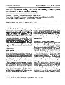
where ws is the weight given to clashing exams scheduled s periods apart. This weighting is then multipled by the number of students involved in the clash. In essence, this means that a bias is given to clashing exams with more students in common so that these are spread further apart. Clashing exams involving fewer students will give a lower overall penalty for a given number of periods apart and are therefore regarded as less important. In this paper we also present results for these same data sets using a simplified objective function which ignores the number of students involved in each clash and therefore weights all clashes equally, whether they have just 1 student in common or 100. Both of these objective functions can be viewed as being worthwhile from different perspectives and give rise to a number of differences in how problems can be regarded as similar or not. The main defining features of the data sets used are given in Table 1. For the purpose of measuring similarity between problems, many other features have to be considered which will have a larger impact on the similarity of two problems. Most of Kyoto, Japan, August 25–28, 2003
??-4
MIC2003: The Fifth Metaheuristics International Conference
Data Set CAR-S-91 CAR-F-92 EAR-F-83 HEC-S-92 KFU-S-93 LSE-F-91 STA-F-83 TRE-S-92 UTA-S-92 UTE-S-92 YOR-F-83
Table 1: Features for Carter Data Sets No. of No. of No. of Conflict Matrix exams students enrollments Density 682 543 181 81 486 381 139 261 622 184 190
16925 18419 1125 2823 5349 2726 611 4360 21267 2750 941
56877 55522 8109 10632 25113 10918 5751 14901 58979 11793 6034
0.13 0.14 0.27 0.20 0.06 0.06 0.14 0.18 0.13 0.08 0.29
No. of periods 35 32 24 18 20 18 13 23 35 10 21
these will come from a statistical analysis of the datasets and their behaviour when various meta-heuristics are applied to them. In the following section we present results of simulated annealing applied to these data sets using both objective functions mentioned above and aim to draw some conclusions regarding how consistent the algorithm is over 10 runs on each problem, how large an impact the initial solution has on the best solution found and how the different objective functions affect this behaviour.
4
Results & Points to note
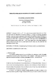
The results presented in this section are taken from 10 runs of our simulated annealing (SA) algorithm on each data set and for each optimisation function. The initial solution to be fed to the SA heuristic is given by a largest degree graph colouring heuristic with backtracking which gives a feasible solution. Our SA heuristic selects moves from a neighbourhood defined by moving an exam, e, from one period, p1 to another, p2 . The exam and period are both chosen at random and only moves leading to a feasible solution are allowed. The chosen feasible move is accepted or rejected using the standard probabilistic acceptance criteria of SA with improving moves always accepted and moves leading to an inferior solution accepted with decreasing probabilty based on a geometric cooling schedule. The starting temperature and cooling schedule were selected at random and tuned based on the results produced. A number of improvements can be made to improve the perfomance of our SA heuristic, but for our purposes the results produced are of an acceptable standard for comparing similarity between problems. In Tables 2 & 3, the same initial solution is used for all 20 runs of the SA heuristic for each data set. The first 10 runs (Table 2) were optimised using the original Carter’s function including student weights for clashes (the Weighted Set), whilst the second set of 10 runs (Table 3) was optimised using the simplified function weighting all clashes based purely on distance apart in the timetable. The values given for Initial Solution in Tables 2 & 3 for a Kyoto, Japan, August 25–28, 2003
MIC2003: The Fifth Metaheuristics International Conference
??-5
Table 2: Results from our Simulated Annealing heuristic initialised by the same solution each time, using the standard Carter’s optimisation function Data Initial Percentage Standard Average Final Set Solution Improvement Deviation Solution CAR-S-91 CAR-F-92 EAR-F-83 HEC-S-92 KFU-S-93 LSE-F-91 STA-F-83 TRE-S-92 UTA-S-92 UTE-S-92 YOR-F-83
160224 141506 63933 53598 190237 56393 101100 59256 141809 116735 49698
22.2% 24.8% 11.1% 22.9% 47.0% 20.0% 3.4% 15.7% 18.3% 31.8% 9.3%
1.02% 1.43% 1.49% 1.81% 2.22% 0.95% 0.68% 1.54% 1.02% 2.44% 1.04%
124648 106367 56846 41308 100790 45125 97701 49944 115827 79587 45073
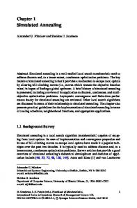
given data set represent the exact same solution, but measured by the two different functions. Tables 4 & 5 show results when a different initial solution is fed to the SA heuristic for each of the 20 runs across the two objective functions. Table 4 using the Carter’s function, Table 5 using the simplified function. For these experiments, a number of other statistics are also noted in addition to those also used in Tables 2 & 3. Due to space constraints, some words in Tables 4 & 5 were abbreviated as follows: Avg. = Average, Init. = Initial, Soln. = Solution, Imp. = Improvement, Std Dev = Standard Deviation. Of course, 10 runs for each data set and optimisation function is not statistically representative. However, in this phase of the research work we aim to provide a guideline for further research and intend to perform more runs in further experiments. The obtained results do provide some interesting points for deeper study since the standard deviations will still be of the same order for a larger number of runs. The results presented for Standard Deviation are calculated as a percentage of the average for a given set of results. It is also worth noting that the initial solution used for each data set in the first set of experiments may be either good or bad so any absolute analysis of the percentage improvement from this solution is not worthwhile. The second set of experiments from 10 different initial solutions each time aims to overcome any bias from a bad or good initial solution. From the results presented in Tables 2 & 3, it can be seen that in all but one case, the SA heuristic improves from the same initial solution 10 times to within a standard deviation of just 3% from the average, indicating that the data sets are relatively stable with respect to our SA heuristic, i.e. when seeded with the same initial solution, the results produced are consistent over 10 runs without huge variations. The one exception to this is the STA-F-83 data set when optimised using the simplified function eliminating student weightings which gives a standard deviation of > 6%. Referring to Table 5, we can see that this behaviour is still apparent Kyoto, Japan, August 25–28, 2003
??-6
MIC2003: The Fifth Metaheuristics International Conference
Table 3: Results from our Simulated Annealing heuristic initialised by the same solution each time, using the simplified optimisation function without student weights Data Initial Percentage Standard Average Final Set Solution Improvement Deviation Solution CAR-S-91 CAR-F-92 EAR-F-83 HEC-S-92 KFU-S-93 LSE-F-91 STA-F-83 TRE-S-92 UTA-S-92 UTE-S-92 YOR-F-83
51091 38634 11316 4329 17616 14613 6193 16194 41331 8366 13392
20.0% 21.6% 12.3% 6.5% 23.8% 29.5% 25.3% 19.9% 25.2% 22.0% 10.7%
0.70% 0.90% 1.20% 1.10% 0.70% 1.00% 6.80% 1.30% 0.90% 2.60% 1.20%
40873 30289 9924 4048 13423 10302 4626 12971 30916 6525 11959
Table 4: Results from our Simulated Annealing heuristic initialised by a different solution each time, using the standard Carter’s optimisation function
Data Set
Avg. Init. Soln.
Std Dev
% Imp.
Std Dev
Avg. Final Soln.
Std Dev
Best Imp.
Best Solution
% imp. for Best Solution
CAR-S-91 CAR-F-92 EAR-F-83 HEC-S-92 KFU-S-93 LSE-F-91 STA-F-83 TRE-S-92 UTA-S-92 UTE-S-92 YOR-F-83
152278 141332 65586 55412 161601 57986 106717 58615 128946 116636 50142
3.33% 2.95% 4.57% 8.27% 10.77% 3.60% 2.89% 3.95% 4.06% 10.50% 2.03%
24.1% 23.5% 15.0% 20.5% 36.1% 25.2% 6.40% 13.1% 20.9% 24.1% 12.0%
2.22% 3.66% 3.32% 10.13% 11.85% 4.31% 1.45% 1.71% 2.60% 6.29% 2.98%
115633 108023 55676 43730 102115 43362 96564 50953 102074 82680 44109
3.94% 3.09% 3.58% 3.21% 3.89% 4.87% 2.71% 3.77% 5.61% 4.64% 3.12%
27.8% 27.8% 20.0% 33.3% 47.2% 30.5% 8.9% 16.3% 24.5% 31.3% 16.6%
110476 101866 52827 40413 98688 37764 96564 48234 90914 82680 42001
27.8% 25.9% 13.9% 31.6% 40.6% 30.5% 5.1% 12.8% 24.5% 19.7% 16.6%
Kyoto, Japan, August 25–28, 2003
MIC2003: The Fifth Metaheuristics International Conference
??-7
Table 5: Results from our Simulated Annealing heuristic initialised by a different solution each time, using the simplified optimisation function without student weights
Data Set
Avg. Init. Soln.
Std Dev
% Imp.
CAR-S-91 CAR-F-92 EAR-F-83 HEC-S-92 KFU-S-93 LSE-F-91 STA-F-83 TRE-S-92 UTA-S-92 UTE-S-92 YOR-F-83
51589 38339 11794 4425 17355 14959 6025 15749 41770 8039 13270
1.30% 1.32% 2.21% 3.19% 1.98% 2.02% 4.18% 1.87% 1.25% 5.19% 1.80%
20.7% 21.5% 14.5% 7.0% 25.4% 30.9% 18.3% 18.9% 25.4% 25.4% 10.8%
Std Dev
Avg. Final Soln.
Std Dev
Best Imp.
Best Solution
% imp. for Best Solution
1.25% 0.93% 2.20% 3.34% 1.62% 2.30% 8.55% 3.02% 1.81% 5.08% 2.68%
40908 30094 9938 4114 12939 10332 4917 12775 31145 5997 11832
1.23% 1.21% 1.32% 2.94% 1.63% 1.50% 8.95% 1.73% 0.90% 7.02% 1.92%
22.0% 22.7% 17.5% 12.6% 27.1% 34.5% 29.3% 23.8% 28.3% 33.0% 14.4%
39994 29616 9938 3926 12590 10034 4167 12335 30542 5253 11338
22.0% 21.4% 14.9% 9.8% 27.1% 34.5% 29.3% 23.8% 28.3% 30.6% 14.4%
when 10 different initial solutions are used, whereas with the Carter’s optimisation function, Table 4 confirms that this same data set is at least as stable as the rest. This indicates that the function used to optimise the data set (i.e. the definition of what a good timetable is) can have a major effect on the consistency of results produced by the algorithm, indicating that this particular data set is similar in behaviour to others when using one function, but very different when using a different function. It can also be noted from Table 5 that this data set shows very different behaviour from the rest when considering the variation of initial solutions vs final solutions. In most cases the standard deviation of the initial solutions and final solutions are fairly similar, yet for the STA-F-83 data set, the SA heuristic introduces a large amount of further variation into the final solution than was present in the 10 initial solutions. From Table 4, we can see that when a variety of initial solutions are used to seed the SA heuristic, the HEC-S-92 and KFU-S-93 data sets suddenly start to produce a much wider range of final solutions with standard deviations of the order of 10%. In the case of the KFU-S-93 data set, it can be seen that the initial solution used in Table 2 was very bad relative to the average initial solution used in Table 4. This, together with the high deviation in initial solutions for this data set helps to explain why the % improvments are so varied. Likewise the HEC-S-92 and UTE-S-92 data sets show a wider range of initial solutions leading to a wider range of % improvements. Despite this though, the Average Final Solutions produced in Table 4 show similar deviations over all data sets. This indicates that although the initial solutions for some data sets show a higher variation, the SA heuristic flattens this out when producing the final solutions by improving the worse initial solutions notably more than the better ones. It is also interesting to note from Tables 4 & 5 that the best final solution and the best percentage improvement for a given data set come from the same run (initial solution) in a large number of cases1 . Further research with more runs would need to be done before any 1
Each run takes between 10 seconds and 3 minutes depending on the data set
Kyoto, Japan, August 25–28, 2003
??-8
MIC2003: The Fifth Metaheuristics International Conference
conclusions can be drawn from this, but it does indicate that in many circumstances, the best solution that the algorithm can find comes from a large improvement from the initial solution rather than from the best initial solution. Analysis of the individual runs for these data sets does indeed show that in many cases some of the best final solutions come from the worst initial solutions. For other data sets though this is markedly not the case and the better final solutions generally come from the better initial solutions indicating a much stronger dependence on having a good initial solution for these data sets in order for the SA heuristic to perform well. In the case of the LSE-F-91 data set in Table 4, the biggest improvement from an initial solution actually comes from the best initial solution yielding a final solution far better than in any of the other 9 runs. This may just be an anomoly of the small number of runs used, but is certainly worthy of further investigation. Finally, when comparing results across the two objective functions it can be seen that there are some very striking differences between certain data sets. Most notably, the HEC-S-92 and KFU-S-93 data sets are improved a great deal more from all the initial solutions when optimised using the standard Carter function than when optimised using the simplified function. On the other hand, the LSE-F-91, STA-F-83 and TRE-S-92 data sets show completely the opposite behaviour and are improved more from an initial solution using the simplified objective function than the standard Carter’s objective function. This again indicates that when measuring similarity between two data sets, the objective function used has a major impact.
5
Conclusions
To conclude, it can be seen from our results that there are a number of interesting differences in the behaviour of some of the data sets when compared against each other for the same objective function and also when compared with the same data set optimised using a different objective function. Since these results are all produced from sets of just 10 runs, further tests will need to be done with many more runs in order to come to any solid conclusions, but our initial results indicate many areas in which this further analysis can be done and provide very worthwhile results. These include further runs of the heuristic on the data sets which provide very varied results (high standard deviation) to see if this is still the same over 100 or more runs, a deeper analysis of the STA-F-83, HEC-S-92, UTE-S-92 and KFU-S-93 data sets to study the large variation in these results when run from 10 different initial solutions and a further examination into exactly which data sets rely strongly on their initial solutions and which produce equivalent quality solutions irrespective of the initial solution. Measuring similarity between two complex optimisation problems is far from an exact science and it will never be possible to say with absolute certainty that two problems are similar and that the heuristic which performs best on one will also perform best on the other, but through our analysis we hope to gain a better understanding of the key factors affecting how similar data sets are with respect to the behaviour of heuristics applied to them. Kyoto, Japan, August 25–28, 2003
MIC2003: The Fifth Metaheuristics International Conference
??-9
References [1] Burke, E.K., Elliman, D.G., Ford, P., Weare, R.F. Examination Timetabling in British Universities - A Survey, in [5] [2] Burke, E.K, Elliman, D.G. and Weare, R.F. A University Timetabling System based on Graph Colouring and Constraint Manipulation Journal of Research on Computing in Education Volume 27 Issue 1 Fall 1994, pages 1-18 [3] Burke, E.K. and Petrovic, S. Recent Research Directions in Automated Timetabling. European Journal of Operational Research - EJOR, 140/2, 2002, 266-280 [4] Burke, E.K., MacCarthy, B., Petrovic, S. and Qu, R. Structured Cases in CBR: Re-using and Adapting Cases for Timetabling Problems. Knowledge-Based Systems 13, pp. 159-165, 2000 [5] Burke, E.K. and Ross, P., editors. Practice and Theory of Automated Timetabling, volume 1153 of Lecture Notes in Computer Science. Springer-Verlag, Berlin, Heidelberg, 1996. [6] Carter, M. W. and Laporte, G. Recent Developments in Practical Examination Timetabling In [5]. [7] Carter, M. W., Laporte, G. and Lee, S. Y. Examination timetabling: Algorithmic strategies and applications. Journal of Operational Research Society, 74:373-383, 1996. [8] Wren, A. Scheduling, timetabling and rostering - A special relationship?. In [5], pp. 46-75.
Kyoto, Japan, August 25–28, 2003