Damian J. J. Farnell and Raymond F. Bishop. Department of Physics, University of Manchester Institute of Science and Technology (UMIST), P.O. Box 88,.
PHYSICAL REVIEW B
VOLUME 61, NUMBER 21
1 JUNE 2000-I
Quantum phase transitions of a square-lattice Heisenberg antiferromagnet with two kinds of nearest-neighbor bonds: A high-order coupled-cluster treatment Sven E. Kru¨ger, Johannes Richter, and Jo¨rg Schulenburg Institut fu¨r Theoretische Physik, Universita¨t Magdeburg, P.O. Box 4120, D-39016 Magdeburg, Germany
Damian J. J. Farnell and Raymond F. Bishop Department of Physics, University of Manchester Institute of Science and Technology (UMIST), P.O. Box 88, Manchester M60 1QD, United Kingdom 共Received 3 August 1999兲 We study the zero-temperature phase diagram and the low-lying excitations of a square-lattice spin-half Heisenberg antiferromagnet with two types of regularly distributed nearest-neighbor exchange bonds 关 J⬎0 共antiferromagnetic兲 and ⫺⬁⬍J ⬘ ⬍⬁兴 using the coupled cluster method 共CCM兲 for high orders of approximation 共up to LSUB8兲. We use a Ne´el model state as well as a helical model state as a starting point for the CCM calculations. We find a second-order transition from a phase with Ne´el order to a finite-gap quantum disordered phase for sufficiently large antiferromagnetic exchange constants J ⬘ ⬎0. For frustrating ferromagnetic couplings J ⬘ ⬍0 we find indications that quantum fluctuations favor a first-order phase transition from the Ne´el order to a quantum helical state, by contrast with the corresponding second-order transition in the corresponding classical model. The results are compared to those of exact diagonalizations of finite systems 共up to 32 sites兲 and those of spin-wave and variational calculations. The CCM results agree well with the exact diagonalization data over the whole range of the parameters. The special case of J ⬘ ⫽0, which is equivalent to the honeycomb lattice, is treated more closely. I. INTRODUCTION
The subject of quantum spin-half antiferromagnetism in low-dimensional systems has attracted a great deal of interest in recent times in connection with the magnetic properties of the cuprate high-temperature superconductors. However, low-dimensional quantum spin systems are of interest in their own right as examples of strongly interacting quantum many-body systems. Although we know from the MerminWagner theorem1 that thermal fluctuations are strong enough to destroy magnetic long-range order at any finite temperature, the role of quantum fluctuations is less understood. As a result of intensive work in the late 1980’s it is now wellestablished that the ground-state of the Heisenberg antiferromagnet on the square lattice with nearest-neighbor interactions is long-range ordered 共see, for example, the review in Ref. 2兲. However, Anderson’s and Fazekas’ investigations3 of the triangular lattice led to a conjecture that quantum fluctuations plus frustration may be sufficient to destroy the Ne´el-like long-range order in two dimensions. Another specific area of recent research is the spin-half J 1 -J 2 antiferromagnet on the square-lattice where the frustrating diagonal J 2 bonds plus quantum fluctuations are able to realize a second-order transition from Ne´el ordering to a disordered quantum spin liquid 共see, for example, Refs. 4–7, and references therein兲. On the other hand, there are cases in which frustration causes a first-order transition in quantum spin systems in contrast to a second-order transition in the corresponding classical model 共see, for example, Refs. 8–11兲. In addition to frustration, there is another mechanism to realize the ‘‘melting’’ of Ne´el ordering in the ground states of unfrustrated Heisenberg antiferromagnets, namely, the formation of local singlet pairs of two coupled spins. This mechanism may be relevant for the quantum disordered state in bilayer systems12–15 as well as in CaV4 O9 共see, for ex0163-1829/2000/61共21兲/14607共9兲/$15.00
PRB 61
ample, Refs. 16–18, and references therein兲. The formation of local singlets is connected with a gap in the excitation spectrum. By contrast, the opening of a gap in the excitation spectrum of frustrated systems seems to be less clear and might be dependent on details of the exchange interactions. In the present paper, we study a model which contains both mechanisms, frustration, and singlet formation, in different parameter regions. We mainly use in this article the coupled cluster method,19–21 which has become widely recognized as one of the most powerful and most universal techniques in quantum many-body theory. In recent years there has been increasing success in applying the CCM to quantum spin systems,7,22–29 especially with the advent of high-order approximations which utilize computer algebra.28 Subsequently, high-order CCM approximations have been applied to the XXZ model,28 the anisotropic XY model,26 and the J 1 -J 2 model.7 In addition to the CCM results we also present variational, spin-wave theory 共SWT兲 and exact diagonalization 共ED兲 results for the sake of comparison. II. THE MODEL
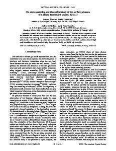
We consider a spin-half Heisenberg model on a square lattice with nearest-neighbor bonds J and J ⬘ in a regular zigzag pattern as shown in Fig. 1. The Hamiltonian is given by
H⫽J
J⫽1
⫽ 14 607
兺
具i j典1
si •s j ⫹J ⬘
兺
具i j典2
si •s j
兺 兺p 关 1⫹ ␦ p,p ⬘共 J ⬘ ⫺1 兲兴 si •si⫹p .
i苸A
J
共1兲
©2000 The American Physical Society
14 608
¨ GER et al. SVEN E. KRU
PRB 61
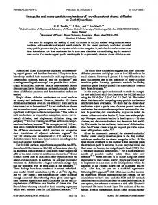
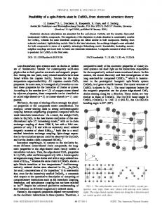
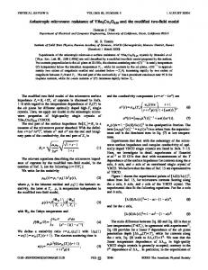
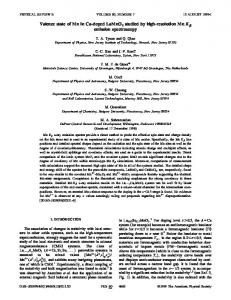
There are some special cases of the model Hamiltonian of Eq. 共1兲. 共i兲 J ⬘ ⫽1: square-lattice antiferromagnet, for which the ground state is long-range ordered; 共ii兲 J ⬘ ⫽0: honeycomb-lattice antiferromagnet, for which the ground state is long-range ordered; 共iii兲 J ⬘ ⫽⫺⬁: spin-1 triangular lattice, for which the ground state is long-range ordered; and 共iv兲 J ⬘ ⫽⫹⬁: valence-bond solid, for which the ground state is a rotationally invariant quantum dimer state with an excitation gap. Classical ground state. For J ⬘ ⬎⫺1/3 the Ne´el state is the classical ground state of the Hamiltonian of Eq. 共1兲. At J ⬘c ⫽⫺1/3 there is classically a second-order phase transition to a ground state of helical nature 共see Fig. 1兲, with a characteristic pitch angle ⌽⫽⫾ 兩 ⌽ cl兩 given by FIG. 1. Illustration of the classical helical state for the squarelattice Heisenberg antiferromagnet of Eq. 共1兲, with two kinds of regularly distributed nearest-neighbour exchange bonds J 共dashed lines兲 and J ⬘ 共solid lines兲. The spin orientations at A and B lattice sites are defined by the angles n ⫽n⌽ and n ⫽n⌽⫹ , respectively, where n⫽0,1,2, . . . , and ⌽ is the characteristic angle of the helical state. The state is shown for ⌽⫽ /12 and n⫽0,1, . . . ,7.
The sums over 具 i j 典 1 and 具 i j 典 2 represent sums over the nearest-neighbor bonds shown in Fig. 1 by dashed and solid lines, respectively. Throughout the paper we fix the J bond to be antiferromagnetic (J⬎0) and henceforth scale it to the value J⫽1, and consider J ⬘ as the free parameter of the model. We also split the square lattice into the equivalent A and B sublattices shown in Fig. 1. In Eq. 共1兲 the sum over i runs over the sites of the sublattice A, with vectors p⫽ 兵 (0, ⫾1),(⫾1,0) 其 connecting nearest neighbors. In particular, p J ⬘ ⫽(1,0) pertains to the coupling with J ⬘ bonds. Each square lattice plaquette consists of three J⫽1 bonds and one J ⬘ bond. In the case of ferromagnetic J ⬘ bonds 共i.e., J ⬘ ⬍0), the plaquettes are frustrated. Conversely, for antiferromagnetic J ⬘ bonds 共i.e., J ⬘ ⬎0) there is no frustration in the system, although the difference of the coupling strengths J and J ⬘ leads to quantum competition. This model has been treated previously using perturbation theory,30 renormalized spin wave theory 共RSWT兲,31 and exact diagonalization 共ED兲.32 It allows us to study the influence of local singlet formation (J ⬘ ⬎1) and frustration (J ⬘ ⬍0) on the stability of the Ne´el order within a single model. Ferromagnetic bonds in an antiferromagnetic matrix have been discussed in recent times4,33–36 in connection with the proposal by Aharony and co-workers37 to model localized oxygen holes in the Cu-O-planes by local ferromagnetic bonds between the copper spins. It was argued that random ferromagnetic bonds may influence the antiferromagnetic order drastically and may support the realization of a quantum spin-liquid state.4,35,36 On the other hand, the case of antiferromagnetic J ⬘ bonds with J ⬘ ⬎1 resembles the situation in bilayer systems and in the depleted square-lattice antiferromagnet CaV4 O9 , in which the competition between two different antiferromagnetic bonds leads to a phase transition from antiferromagnetic long-range order to quantum disorder with a finite gap. It is seen in this article that the transition point obtained for the model of Eq. 共1兲 is quite close to that obtained for the bilayer model.13
兩 ⌽ cl兩 ⫽
冦
0
1 J ⬘ ⬎⫺ , 3
arccos
冉冑 冊 1 2
1⫺
1
J⬘
1 J ⬘ ⭐⫺ , 3
共2兲
where the different signs correspond to the two chiralities38 of this helical state. Note that for ⌽⫽0 this is just the Ne´el state. More generally, the pitch angle varies with J ⬘ from 兩 ⌽ cl兩 ⫽0 for J ⬘ ⬎⫺1/3 to 兩 ⌽ cl兩 ⫽ /3 for J ⬘ ⫽⫺⬁. Note that 兩 ⌽ cl兩 ⫽ /3 共realized at J ⬘ ⫽⫺⬁) corresponds to the ground state of the spin-1 triangular lattice. We describe the directions of the spins sA and sB , belonging to the A and B sublattices respectively, for the classical helical state with a characteristic angle ⌽ as follows31 共and see Fig. 1兲, sA 共 R兲 ⫽uˆ cos Q•R⫹vˆ sin Q•R,
共3兲
sB 共 R⫹xˆ 兲 ⫽uˆ cos共 Q•R⫹ ⫹3⌽ 兲 ⫹vˆ sin共 Q•R⫹ ⫹3⌽ 兲 , where uˆ and vˆ are perpendicular unit vectors in the spin space, R runs over the sites of the sublattice A, and we have Q⫽(2⌽,0) for the pitch vector Q. We note that this general helical state does not have a periodicity in the x direction because ⌽ is in general not of the form m /n with m and n integral. We also note that we have only three different angles between nearest-neighbor spins, namely, ⫾( ⫺⌽) for the J⫽1 couplings and ⫺3⌽ for the coupling with J ⬘ . The maximum frustration is in the region around J ⬘ ⬇ ⫺1. Bearing in mind the situation for the J 1 -J 2 model, one might expect that for the extreme quantum case 共spin-half兲 quantum fluctuations might be able to open the window to a spin-liquid phase for a finite range of parameters around this region of maximum frustration. On the other hand, for strong antiferromagnetic bonds (J ⬘ Ⰷ1) there is, of course, no indication in the classical model for the breakdown of the Ne´el order. Simple variational ansatz for the quantum ground state. In the quantum case, the region of strong antiferromagnetic J ⬘ bonds (J ⬘ Ⰷ1) is characterized by a tendency to singlet pairing of the two spins corresponding to a J ⬘ bond. Using a high-order series expansion30 the Ne´el order was found to be stable up to a critical value J s⬘ ⬇2.56.
PRB 61
QUANTUM PHASE TRANSITIONS OF A SQUARE- . . .
A comparable value can be obtained using a simple variational wave function similar to that used14 for bilayer systems, namely,
兩 ⌿ var典 ⫽
1
关 兩 ↑ i ↓ i⫹xˆ 典 ⫺t 兩 ↓ i ↑ i⫹xˆ 典 ], 兿 i苸A 冑1⫹t 2
共4兲
where the lattice sites i and i⫹xˆ correspond to a J ⬘ bond, and where the product in Eq. 共4兲 is thus effectively taken over the J ⬘ bonds of the lattice of Eq. 共1兲. The trial function depends on the variational parameter t and interpolates between a valence-bond state realized for t⫽1 and the Ne´el state for t⫽0. For t⫽1, the singlet pairing is complete and 兩 ⌿ var典 represents an eigenstate of the model of Eq. 共1兲 in the limit J ⬘ →⬁ 共dimer state兲. By minimizing 具 ⌿ var兩 H 兩 ⌿ var典 with respect to the variational parameter t we get an upper bound for the ground-state energy per spin of the model of Eq. 共1兲,
再
⫺ 共 J ⬘ 2 ⫹3J ⬘ ⫹9 兲 /24,
E var /N⫽ ⫺3J ⬘ /8,
J ⬘ ⭐3,
J ⬘ ⬎3.
共5兲
The relevant order parameter describing the Ne´el order is
M var⫽ 具 ⌿ var兩 s zi 兩 ⌿ var典 ⫽
再
1/2冑1⫺J ⬘ 2 /9, 0,
J ⬘ ⭐3,
J ⬘ ⬎3.
兩 ⌽ 典 ⫽ 兩 •••↓↓↓••• 典 ,
The starting point for any CCM calculation 共see overwiew in Ref. 21兲 is the choice of a normalized model or reference state 兩 ⌽ 典 , together with a set of mutually commuting multispin creation operators C I⫹ which are defined over a complete set of many-body configurations I. The operators C I are the multispin destruction operators and are defined to be the Hermitian adjoints of the C I⫹ . We choose 兵 兩 ⌽ 典 ;C I⫹ 其 in such a way that we have 具 ⌽ 兩 C I⫹ ⫽0⫽C I 兩 ⌽ 典 , ᭙I⫽0, where, by definiton, C ⫹ 0 ⫽1, the identity operator. For spin systems, an appropriate choice for the CCM model state 兩 ⌽ 典 is often a classical spin state,23 in which the most general situation is that each spin can point in an arbitrary direction. For the case of the Hamiltonian of Eq. 共1兲, we choose the helical state illustrated in Fig. 1 to be our model state. Although the classical ground state of Eq. 共1兲 is precisely of this form, we do not choose the classical result for the pitch angle ⌽ but we consider it rather as a free parameter in the CCM calculation. In order to perform a CCM calculation, we would like to treat each site equivalently and we do this by performing a rotation of the local spin axes at each site about the y axis such that all spins in the model state align in the same direction, say down 共along the negative z axis兲. After this transformation we have
⫹ ⫹
共7兲
s xi →cos ␦ i s xi ⫹sin ␦ i s zi , s iy →s iy ,
共8兲
s zi →⫺sin ␦ i s xi ⫹cos ␦ i s zi . A similar rotation about the y-axis by an angle ␦ j is performed for the spin s j . Thus we get for the transformation of the scalar product of the two spins si •s j →(si •s j ) , where 共 si •s j 兲 ⬅sin 关 s xi s zj ⫺s zi s xj 兴 ⫹cos 关 s xi s xj ⫹s zi s zj 兴 ⫹s iy s yj
1 z z ⫹ ⫺ z z ⫺ z z ⫽ sin 关 s ⫹ i s j ⫺s i s j ⫹s i s j ⫺s i s j 兴 ⫹cos s i s j 2 1 ⫺ ⫺ ⫹ ⫹ 共 cos ⫹1 兲关 s ⫹ i s j ⫹s i s j 兴 4
showing a breakdown of the Ne´el order at a critical value J s⬘ ⫽3.
A. The ground-state formalism
⫹
C I⫹ ⫽s r⫹ ,s r⫹ s r ⬘ ,s r⫹ s r ⬘ s r ⬙ , . . . ,
共where the indices r,r ⬘ ,r ⬙ , . . . denote any lattice site兲 respectively, for the model state and the multispin creation operators, which now consist of spin-raising operators only. In order to make the spin si point down let us suppose we need to perform such a rotation of the spin axes by an angle ␦ i . This is equivalent to the transformation
共6兲
III. COUPLED CLUSTER CALCULATIONS
14 609
1 ⫹ ⫺ ⫺ ⫹ 共 cos ⫺1 兲关 s ⫹ i s j ⫹s i s j 兴 . 4
共9兲
The angle ⬅ ␦ j ⫺ ␦ i is the angle between the two spins, and s ⫾ ⬅s x ⫾is y are the spin-raising and spin-lowering operators. Note that this product of two spins after the rotation depends not only on the angle between them, but also on the sign of this angle. In case of the Ne´el model state (⌽⫽0), the angle between any neighboring spins is , and hence Eq. 共9兲 be⫹ ⫺ ⫺ z z comes si •s j →⫺ 21 关 s ⫹ i s j ⫹s i s j 兴 ⫺s i s j . Using the helical state of Eq. 共3兲 with the characteristic angle ⌽, the Hamiltonian of Eq. 共1兲 is now rewritten in the local coordinates as
H⫽
兺 兺p 关 1⫹ ␦ p,p ⬘共 J ⬘ ⫺1 兲兴共 si •si⫹p 兲 ,
i苸A
J
p
共10兲
where the angles between neighboring spins are ⫾yˆ ⫽ ⫹⌽, ⫺xˆ ⫽ ⫺⌽ and xˆ ⫽ ⫹3⌽. While the general helical state 共see Fig. 1兲 does not have translational symmetry in the x direction, the transformed Hamiltonian of Eq. 共10兲 does have this symmetry since it depends only on the angles between neighboring spins. Having defined an appropriate model state 兩 ⌽ 典 with creation operators C I⫹ , the CCM parametrizations of the ket and bra ground states are given by 兩 ⌿ 典 ⫽e S 兩 ⌽ 典 ,
S⫽
兺
I⫽0
SI C I⫹ ,
共11兲
¨ GER et al. SVEN E. KRU
14 610
˜ 兩 ⫽ 具 ⌽ 兩˜S e ⫺S , 具⌿
˜S ⫽1⫹
兺 ˜SI C I . I⫽0
共12兲
The correlation operator S is expressed in terms of the creation operators C I⫹ and the ket-state correlation coefficients SI . We can now write the ground-state energy as E⫽ 具 ⌽ 兩 e ⫺S He S 兩 ⌽ 典 .
共13兲
To describe the magnetic order of the system, we use a simple order parameter which is expressed in terms of the local, rotated spin axes, and which is given by ˜ 兩 s zi 兩 ⌿ 典 , M ⬅⫺ 具 ⌿
共14兲
such that the order parameter represents the on-site magnetization. Note that M is the usual sublattice magnetization for the case of the Ne´el state as the CCM model state. To find the ket-state and bra-state correlation coefficients ¯ ⫽具⌿ ˜ 兩H兩⌿典 we have to require that the expectation value H is a minimum with respect to the bra-state and ket-state correlation coefficients. This formalism is exact if we include all possible multispin configurations in the correlation operators S and ˜S , which is usually impossible in a practical situation. We use the LSUBn approximation scheme28 to truncate the expansion of S and ˜S in Eqs. 共11兲 and 共12兲. Using the lattice symmetries, we have now to find all different possible configurations with respect to the point and space group symmetries of both the lattice and Hamiltonian with up to n spins spanning a range of no more than n adjacent lattice sites 共LSUBn approximation兲 and these are referred to as the fundamental configurations. The Hamiltonian of Eq. 共1兲 has four lattice point-group symmetries, namely, two rotational operations (0°,180°) and two reflections 共along the x and y axes兲, defined by x→x,
y→y,
x→x,
y→⫺y,
x→⫺ 共 x⫹1 兲 , x→⫺ 共 x⫹1 兲 ,
共15兲
The rotation of 180° and the reflection along the y-axis are connected by a shift of xˆ ⫽(1,0). The translational operator T is defined by T⫽ 共 n⫹m 兲 xˆ ⫹ 共 m⫺n 兲 yˆ ,
n,m integral,
TABLE I. Number of fundamental ground-state configurations of the LSUBn approximation for the Hamiltonian of Eq. 共1兲, using a Ne´el state (⌽⫽0) and a helical state (⌽⫽0) for the CCM model state, and the number of fundamental excited state configurations using the Ne´el model state only. LSUBn
ground state: ⌽⫽0
⌽⫽0
excited state: ⌽⫽0
2 4 6 8
3 22 267 4986
5 76 1638 42160
1 16 331 7863
we exclude configurations with an odd number of spins, and therefore we do not use LSUB3, LSUB5, etc., approximations. The helical state is not an eigenstate of s Tz and we cannot apply this property when using the helical model state. The fundamental configurations can now be calculated computationally,28 and the resulting numbers of LSUBn configurations for n⭐8 are given in Table I. The ket-state and bra-state equations are calculated computationally.28 For the Ne´el model state, we are able to carry out the CCM up to the LSUB8 level 共where we need to solve 4986 coupled equations兲, whereas for the helical state we could do this only up to the LSUB6 level 共where we need to solve 1638 coupled equations兲. B. The excited state formalism
We use the excited-state formalism of Emrich39,23,40 to approximate the excited-state wave functions. We apply an excitation operator X e linearly to the ket state wave function 共11兲, such that 兩 ⌿ e 典 ⫽X e e S 兩 ⌽ 典 ,
X e⫽
兺
I⫽0
X Ie C I⫹ .
共17兲
Using the Schro¨dinger equation H 兩 ⌿ e 典 ⫽E e 兩 ⌿ e 典 , we find that
y→⫺y, y→y.
PRB 61
共16兲
such that translational symmetry is preserved. The Ne´el model state also contains these symmetries, and so for this model state we can directly apply all these symmetries in finding the fundamental configurations. On the other hand the general helical model state (⌽⫽0) has only two of the above four lattice point-group symmetries, namely, x→x, y→y, and x→x, y→⫺y, and so this reduced symmetry yields a larger number of fundamental configurations. In the case of the Ne´el model state (⌽⫽0), the number of fundamental configurations can further be reduced by explicitly conserving the total uniform magnetization s Tz ⬅ 兺 k s zk 共the sum on k runs over all lattice sites兲 because the ground state is known to lie in the s Tz ⫽0 subspace. This means that
⑀ e X e 兩 ⌽ 典 ⫽e ⫺S 关 H,X e 兴 ⫺ e S 兩 ⌽ 典 ,
共18兲
where ⑀ e (⬅E e ⫺E) is the difference between the excitedstate energy (E e ) and the ground-state energy (E). Applying 具 ⌽ 兩 C I to Eq. 共18兲 we find that
⑀ e X Ie ⫽ 具 ⌽ 兩 C I e ⫺S 关 H,X e 兴 ⫺ e S 兩 ⌽ 典 ,
共19兲
which is an eigenvalue equation with eigenvalues ⑀ e and corresponding eigenvectors X Ie . As for the ground state, we must use an approximation scheme for X e in Eq. 共17兲. Although it is not necessary40 to use the same approximation for the excited state as for the ground state, we in fact do so to keep the CCM calculations as systematic and self-consistent as possible. We define the fundamental configurations for LSUBn 共for the Ne´el state兲 as previously, but we now restrict the choice of configurations to contain only those which produce a change of s Tz of ⫾1 with respect to the model state.40 Since we are only interested in the lowest-lying excitations, the restriction to these single-magnon spin-wave-like excitations is the correct
PRB 61
QUANTUM PHASE TRANSITIONS OF A SQUARE- . . .
choice. The number of fundamental excited-state configurations for LSUBn is given in Table I. To calculate the terms of the right hand side of Eq. 共19兲 we use the same computational algorithm as for the calculation of the ground-state ket equation. The terms contain the ground ket-state correlation coefficients SI , so once these coefficients have been determined the eigenvalue equation 共19兲 can be solved 共numerically兲. We furthermore choose the lowest energy eigenvalue of Eq. 共19兲 in order to calculate the excitation energy gap ⌬. We note that the eigenvalues of Eq. 共19兲 are not guaranteed to be real, since as a generalized eigenvalue equation it is not symmetric. However, over the entire regime of interest, the values of ⌬ so obtained are found to be real. We have performed these calculations for the excited state up to the LSUB6 level of approximation. C. Extrapolation of the CCM-LSUBn results
Although no scaling theory for results of LSUBn approximations has yet been proven, there are empirical indications24,26,28,40 of scaling laws for the energy, the magnetization, and the excited-state energy gap for various spin models. These scaling laws can be justified by the observations that they fit the results well 共i.e., with low mean-square deviation兲, and that the extrapolated results are in good agreement with results of other methods 关e.g., Green function Monte Carlo or series expansion for the two-dimensional 共2D兲 XXZ model24,28兴 or with exact results 共e.g., 1D XY model26兲. In accordance with those previous results we use the following scaling laws: for the ground-state energy, E⫽a 0 ⫹a 1 共 1/n 2 兲 ⫹a 2 共 1/n 2 兲 2 ;
共20兲
for the ground-state magnetization, M ⫽b 0 ⫹b 1 共 1/n 兲 ⫹b 2 共 1/n 兲 2 ;
共21兲
and for the gap of the lowest-lying excitations, ⌬⫽c 0 ⫹c 1 共 1/n 兲 ⫹c 2 共 1/n 兲 2 ;
共22兲
where n is the LSUBn approximation level. D. Choice of the CCM model state
As stated previously, we use the helical state of Eq. 共3兲 with the characteristic angle ⌽, illustrated in Fig. 1, as the model state for the CCM. We must therefore make a selection of an appropriate value for ⌽. A possible choice would be the classical ground state of the Hamiltonian of Eq. 共1兲 关i.e., ⌽⫽⌽ cl as given by Eq. 共2兲兴. Another possibility is to perform a CCM-LSUBn approximation calculation and then to minimize the corresponding LSUBn approximation to the energy with respect to ⌽, E LSUBn 共 ⌽ 兲 →min
⇔
⌽⫽⌽ LSUBn .
共23兲
The results for ⌽ LSUBn will be given later 共Fig. 7兲. However, we note now that although the CCM does not yield a strict upper bound for the ground-state energy, using ⌽⫽⌽ LSUBn 共i.e., using the CCM with a variational parameter兲 has been
14 611
found to be a reasonable assumption.25 There are several additional arguments to suggest that ⌽⫽⌽ LSUBn is indeed a better choice than ⌽⫽⌽ cl , as indicated below. In the first place we note that we cannot find solutions for the LSUB6 equations using ⌽⫽⌽ cl(J ⬘ ) in the region ⫺0.7 ⱗJ ⬘ ⱗ⫺0.47 insofar as the Newton method used to solve these equations does not converge in that region. This is a clear indication that this model state is not a good one. By contrast, such behavior is not found for ⌽⫽⌽ LSUBn . Secondly, it is generally known that quantum fluctuations tend to prefer collinear order4,42 共e.g., Ne´el order兲. We will indeed find 共and see Fig. 7 below兲 that the Ne´el ordering (⌽⫽0) seems to survive for some J ⬘ ⬍⫺1/3, in which region it has already broken down in the classical case. This is also in agreement with results of exact diagonalizations for our model 共and see Fig. 5 below兲. Thirdly we find better agreement of the CCM results for the energy compared to exact diagonalization results by using the helical state as the model state with the value ⌽ ⫽⌽ LSUBn rather than with the classical value ⌽⫽⌽ cl . We find that CCM results for the ground-state energy usually agree well with the corresponding ED results 共and with results of other methods兲,28 provided that a good CCM model state is chosen. We therefore use the helical state with ⌽⫽⌽ LSUBn as the CCM model state throughout this paper. Note that for J ⬘ ⭓ ⫺1/3 this model state is identical to the classical ground state of Eq. 共1兲 but that for J ⬘ ⬍⫺1/3 it is not.
IV. RESULTS
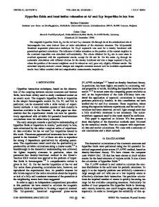
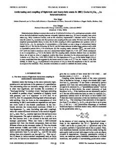
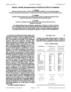
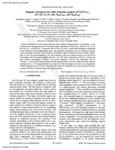
Using the CCM scheme described above, we calculate the approximate ground state and the low-lying excitations of the Hamiltonian of Eq. 共1兲. For comparison we also exactly diagonalize finite sized lattices of square shape. We use periodic boundary conditions with N⫽16,18,20,26, and 32 spins, and we extrapolate to the infinite system using standard finite-size scaling laws.41,42 We present results for the ground-state energy, the order parameter and the excitation gap. We examine the formation of local singlets 共for J ⬘ ⬎1), the effects of frustration 共for J ⬘ ⬍0), and the special case of the honeycomb lattice (J ⬘ ⫽0). J ⬘ ⬎1: Formation of local singlets. Using the CCM we obtain clear indications of a second-order phase transition to a disordered dimerlike phase at a certain critical value of J ⬘ , namely, J s⬘ . For J ⬘ ⬎J s⬘ , the Ne´el-like long range order melts 关i.e., the sublattice magnetization M given by Eq. 共14兲 becomes zero兴. Our estimate for J s⬘ using the four extrapolated LSUBn results for M with n⫽2,4,6,8 共see Fig. 2兲 is J s⬘ ⬇3.41. However, using only the three CCM LSUBn approximations with n⫽4,6,8 for the extrapolation, we obtain a value J s⬘ ⬇3.16, which indicates that the true value could be even somewhat smaller. This is in agreement with our corresponding result using exact diagonalizations of small systems. By using the extrapolation scheme of Ref. 42, we find a critical value J s⬘ ⬇2.45 for the magnetization. Note, however, that better accuracy requires larger systems because of the exact diagonalization 共ED兲 extrapolation ansatz for M 共i.e., M ⫽M ⬁ ⫹const⫻N ⫺1/2). Therefore, we cannot consider the ED results for the magnetization 共and see Fig. 2兲 as
14 612
¨ GER et al. SVEN E. KRU
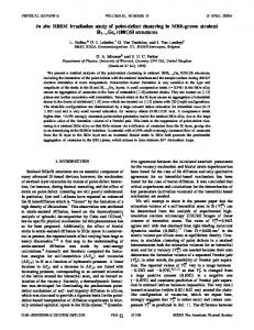
FIG. 2. Ground-state magnetic order parameter 关Eq. 共14兲兴 versus J ⬘ , for the CCM-LSUBn approximation. The results are compared 共for the Ne´el region only兲 with M s (⬁), using exact diagonalization 共ED兲 data of the antiferromagnetic structure factor, using the ansatz M s2 ⫽(1/N 2 ) 兺 i, j (⫺1) i⫹ j 具 si •s j 典 ⫽M s (⬁) 2 ⫹const⫻N ⫺1/2. Note that both extrapolated results fit poorly in a region around J ⬘ ⬇⫺1, and we therefore plot them here as isolated points 共omitting the solid lines兲.
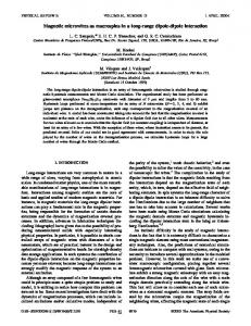
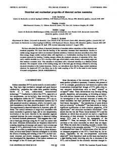
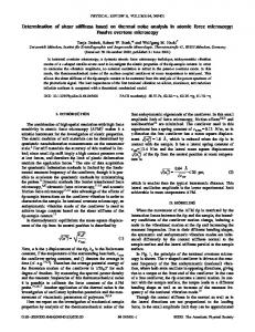
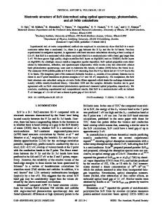
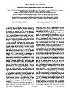
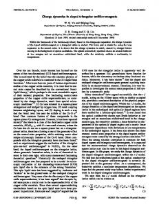
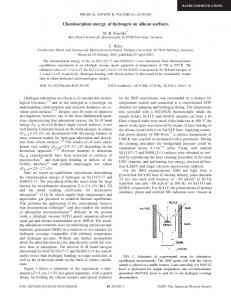
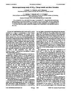
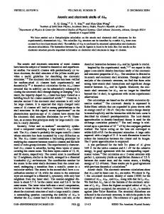
quantitatively correct. Our two results for the critical J s⬘ also agree with the estimate J s⬘ ⬇2.56 from series expansion,30 and even the result J s⬘ ⫽3 from the simple variational ansatz of Eq. 共4兲 agrees surprisingly well with these values. By contrast, the second-order renormalized spin wave theory 共RSWT兲 共Ref. 31兲 gives the larger result J s⬘ ⬇5.0, indicating that the standard spin-wave approach is insufficient to describe this type of transition. Another indication of a dimerized phase is the appearance of a gap ⌬ between the ground state and the lowest-lying excited state. We clearly expect a spectrum with gapless Goldstone modes if the ground state is Ne´el long-range ordered, whereas for a disordered singlet ground-state the formation of triplet excitations may cost a finite amount of energy. This behavior is reflected by our results using both CCM and exact diagonalization 共see Fig. 3兲, which agree well with each other. For J ⬘ ⰇJ s⬘ , there is a gap proportional to J ⬘ , corresponding to the dimerlike nature of the ground state. The gap obviously opens in the range 2.5ⱗJ s⬘ ⱗ3.0 in both the ED and CCM calculations. This is in good agreement with the corresponding estimates for the critical point using the order parameter. Note, that the standard linear spin wave theory fails in calculating the gap 共i.e., gives gapless modes for all values of J ⬘ with J ⬘ ⬎0).31 By comparing the results for the ground-state energy, we find excellent agreement between the CCM results and the results from exact diagonalization 共see Fig. 4兲 for J ⬘ ⬎0. By contrast, spin-wave theory 共SWT兲 calculations31 show a significant deviation from these results for larger J ⬘ Ⰷ1. These spin-wave results are obviously poor since the simple upper bound for the energy given by Eq. 共5兲 共e.g., E 0 ⫽⫺1.5 for J ⬘ ⫽4) is smaller than the corresponding SWT results 共e.g., E 0 ⫽⫺1.42 from second-order RSWT兲. By contrast, CCM and ED results 共both are about E 0 ⫽⫺1.54 for J ⬘ ⫽4) are
PRB 61
FIG. 3. The gap ⌬ between the lowest-lying excitation energy and the ground-state energy versus J ⬘ using the CCM-LSUBn approximations, in comparison with the extrapolated result of exact diagonalization 共ED兲 共using the ansatz ⌬⫽⌬ ⬁ ⫹const⫻N ⫺1 ).
slightly smaller than the variational result. While both CCM and SWT calculations have the Ne´el state as starting point, we find the CCM is much better able than SWT to describe the transition to the rotationally invariant disordered state and to the completely dimerized state 关represented by the variational function of Eq. 共4兲 with t⫽1兴. Note that even the simplest CCM approximation 共LSUB2兲 gives the correct asymptotic result for the energy 关i.e., Eq. 共5兲兴 for very large values of J ⬘ , whereas SWT does not. For the case of the pure square-lattice Heisenberg antiferromagnet 共i.e., J ⬘ ⫽1), we reproduce the CCM results of Refs. 28,40, which have already been demonstrated to agree well with those from other methods. J ⬘ ⫽0: honeycomb lattice. For the special case of J ⬘ ⫽0 共which is equivalent to the honeycomb lattice兲, we find that the CCM and the ED results are in good agreement 共see Table II兲. However, the magnetization M for ED is found to
FIG. 4. Ground-state energy 关Eq. 共13兲兴 versus J ⬘ for the extrapolated CCM-LSUBn approximations, in comparison with results of spin-wave theory 共linear and second-order renormalized兲, 共Ref. 31兲 and with the extrapolated result of exact diagonalization 共ED兲 data 共using the ansatz E/N⫽E ⬁ /N⫹const⫻N ⫺3/2).
PRB 61
QUANTUM PHASE TRANSITIONS OF A SQUARE- . . .
14 613
TABLE II. Ground-state energy per spin, sublattice magnetization, and excitation energy gap for the Hamiltonian of Eq. 共1兲 with J ⬘ ⫽0. This special case is equivalent to the honeycomb lattice. We present 共extrapolated兲 LSUBn results and extrapolated ED results. LSUB2 LSUB4 LSUB6 LSUB8 extrapolated E/N ⫺0.525 ⫺0.540 ⫺0.542 ⫺0.543 M 0.399 0.354 0.334 0.321 gap 1.182 0.678 0.476
⫺0.5447 0.28 0.02
ED ⫺0.543 0.23 0.06
be smaller then the CCM result. We note, however, that the CCM result for M at this point agrees with the result of high-order SWT 共Ref. 31兲 (M ⫽0.28) as well as with the result of series expansion43 (M ⫽0.26), although it does not agree so well with the result of Monte Carlo calculations44 (M ⫽0.22). We note too that our CCM results here agree perfectly with previous lower-order CCM calculations.27 J ⬘ ⬍0: Frustration. For J ⬘ ⱗ⫺2, we find that the extrapolated ED results for the energy lie appreciably above the CCM 共and SWT兲 results 共see Fig. 4兲. This is because the energies for the small lattices considered do not fit well to the finite-size scaling law (E/N⫽E ⬁ /N⫹const⫻N ⫺3/2) in this region. The finite-size effects for systems with an incommensurate helical structure are found to be larger than for systems with, for example, Ne´el order or with dimerized spin pairs. However, we find that our best ED result 共with 32 spins兲 shows only very small deviations from the CCM result, even in the frustrated region. While classically we have a second-order phase transition 共from Ne´el order to helical order兲 at J ⬘c ⫽⫺1/3, using the CCM we find indications for a shift of this critical point to a value J ⬘c ⬇⫺1.35 共see Fig. 7兲 below in the quantum case. The ED data of the structure factors 共see Fig. 5兲 also show a
FIG. 5. Ground-state structure factor S(k)⬀ 兺 i, j苸A e i(R j ⫺Ri )•k具 si •s j 典 共i.e., the summation is taken over one sublattice兲 for the Hamiltonian of Eq. 共1兲 with 32 spins, for the quantum and the classical case. The Ne´el order 关 k⫽(0,0) 兴 becomes unstable against the helical order in the classical model for J ⬘ ⬍⫺0.5, but in the quantum model the Ne´el ordering gives way to helical order only for J ⬘ ⱗ ⫺1.1 共i.e., the Ne´el ordering is stable quantum-mechanically in a region where it is classically already unstable兲.
FIG. 6. Ground-state energy of the Hamiltonian of Eq. 共1兲 using CCM-LSUB4 versus the parameter ⌽ of the helical CCM model state for certain values of J ⬘ in the range ⫺1.5⭐J ⬘ ⭐⫺1.0. A local minimum of E(⌽) at ⌽⫽0 appears for J ⬘ ⱗ⫺1.1, which for values of J ⬘ ⱗ⫺1.35 becomes a global minimum 关i.e., at ⌽ ⫽⌽ LSUB4 (J ⬘ )兴, indicating the typical scenario of a first-order phase transition. The arrows 共v兲 indicate the value of ⌽ cl for the different values of J ⬘ .
shift of the transition to stronger ferromagnetic J ⬘ bonds. Both correspond to the general picture that quantum fluctuations prefer a collinear ordering 共such as Ne´el order兲. Hence this ordered state can survive for the quantum case into a region where classically it is already unstable. The Ne´el model state (⌽⫽0) gives the minimum ground-state energy for all values J ⬘ ⬎J ⬘c , where J c⬘ is also dependent on the level of LSUBn approximation level. For J ⬘ ⬍J c⬘ another minimum in the energy for ⌽⫽0 is found to lie lower than the minimum at ⌽⫽0 共see Fig. 6兲. The state for ⌽⫽0 is believed to be a quantum analog of the classical ground state in two dimensions. Furthermore, the crossover from one minimum solution to the other is not smooth but is abrupt at this point 共see Fig. 6 and Fig. 7兲. This behavior is assumed here to be an indication of a phase transition. Furthermore, it might also indicate that this is a first-order phase transition and, consequently, that due to quantum fluctuations the nature of this phase transition is changed from the classical second-order type to a first-order type. The behavior of the order parameter 共see Fig. 2兲 in the region around J ⬘c ⬇⫺1.35 where we expect the abovementioned quantum phase transition is also quite marked. We cannot extrapolate the LSUBn results directly, because the phase transition points shift with the order of the LSUBn approximations 共Fig. 7兲. We thus find a large statistical deviation of the extrapolated results in the region ⫺1.4ⱗJ ⬘ ⱗ ⫺1.0. Hence, we use the minima for M in that region to extrapolate an estimation of the order parameter. We find that minimum (M ⬇0.05) to be at a value of J ⬘ ⬇⫺1.2. The extrapolated ED results do not agree very well with this result, since these give M to be zero at J ⬘ ⬇⫺0.8. However, these results are also very poor in that region because of the strong influence of the boundary conditions and large statistical errors. As a result of these difficulties we are not able to decide whether or not quantum fluctuations and frustration are able to form a disordered quantum spin liquid phase 共i.e., with M ⫽0) between the Ne´el state and the helical state for
14 614
¨ GER et al. SVEN E. KRU
PRB 61 V. SUMMARY
FIG. 7. The angle ⌽ LSUBn 关which minimizes the energy E(⌽), see Eq. 共23兲兴 versus J ⬘ , compared with the corresponding classical result ⌽ cl 关see Eq. 共2兲兴. We find in the quantum case 共LSUBn) a first-order phase transition 共e.g., for LSUB6 at J ⬘ ⬇⫺1.35 where ⌽ LSUBn jumps discontinuously from zero to about 0.65兲. By contrast, in the classical case a second-order transition occurs at J ⬘ ⫽⫺1/3.
some finite frustrating J ⬘ ⬍0 regime. However, the CCM results suggest that there is either no quantum spin liquid phase or that, if it does exist, it does so only in a very small region.
N. Mermin and H. Wagner, Phys. Rev. Lett. 17, 1133 共1966兲. E. Manousakis, Rev. Mod. Phys. 63, 1 共1991兲. 3 P.W. Anderson, Mater. Res. Bull. 8, 153 共1973兲; P. Fazekas and P.W. Anderson, Philos. Mag. 30, 423 共1974兲. 4 J. Richter, Phys. Rev. B 47, 5794 共1993兲. 5 A. Chubukov, S. Sachdev, and T. Senthil, Nucl. Phys. B 426, 601 共1994兲. 6 J. Oitmaa and Zheng Weihong, Phys. Rev. B 54, 3022 共1996兲. 7 R.F. Bishop, D.J.J. Farnell, and J.B. Parkinson, Phys. Rev. B 58, 6394 共1998兲. 8 Y. Xian, Phys. Rev. B 52, 12 485 共1995兲. 9 H. Niggemann, G. Uimin, and J. Zittartz, J. Phys.: Condens. Matter 9, 9031 共1997兲. 10 J. Richter, N.B. Ivanov, and J. Schulenburg, J. Phys.: Condens. Matter 10, 3635 共1998兲. 11 N.B. Ivanov, J. Richter, and U. Schollwo¨ck, Phys. Rev. B 58, 14 456 共1998兲. 12 A.J. Millis and H. Monien, Phys. Rev. Lett. 70, 2810 共1993兲. 13 A.W. Sandvik and D.J. Scalapino, Phys. Rev. Lett. 72, 2777 共1994兲. 14 C. Gros, W. Wenzel, and J. Richter, Europhys. Lett. 32, 747 共1995兲. 15 A.V. Chubukov and D.K. Morr, Phys. Rev. B 52, 3521 共1995兲. 16 M. Troyer, H. Kontani, and K. Ueda, Phys. Rev. Lett. 76, 3822 共1996兲; M. Troyer, M. Imada, and K. Ueda, J. Phys. Soc. Jpn. 66, 2957 共1997兲. 17 S. Sachdev, and N. Read, Phys. Rev. Lett. 77, 4800 共1996兲.
Using the CCM we have studied the influence of quantum spin fluctuations on both the ground-state phase diagram and the excited states of a spin-half square-lattice Heisenberg antiferromagnet with two kinds of nearest-neighbor exchange bonds. The phase diagram is found to contain a quantum helical phase, a Ne´el ordered phase, and a finite-gap quantum disordered phase. While we have clearly a second-order transition from the Ne´el phase to the finite-gap quantum disordered phase, we also found indications of a quantum-induced first-order transition from the Ne´el phase to the helical phase, for which classically we have a second-order transition. While our CCM results were in general in good agreement with the ED data, we found the CCM particularly good at describing the dimerized phase. By contrast, spin wave theory31 fails in that region due to enhanced longitudinal spin fluctuations. Accurate high-order CCM results for the antiferromagnet on the honeycomb lattice were also presented.
ACKNOWLEDGMENTS
We would like to thank N.B. Ivanov for his stimulating discussions. This work has also been supported in part by the Deutsche Forschungsgemeinschaft 共GRK 14, Graduiertenkolleg on ‘‘Classification of Phase Transitions in Crystalline Materials’’兲, and by research Grant No. GR/M45429 from the Engineering and Physical Sciences Research Council 共EPSRC兲 of Great Britain.
M. Albrecht and F. Mila, Phys. Rev. B 53, R2945 共1996兲. F. Coester, Nucl. Phys. 7, 421 共1958兲; F. Coester and H. Ku¨mmel, ibid. 17, 477 共1960兲. 20 R.F. Bishop and H. Ku¨mmel, Phys. Today 40共3兲, 52 共1987兲. 21 R.F. Bishop, Theor. Chim. Acta 80, 95 共1991兲; R. F. Bishop, in Microscopic Many-Body Theories and Their Applications, edited by J. Navarro and A. Polls, Vol. 510 of Lecture Notes in Physics 共Springer-Verlag, Berlin, 1998兲, p. 1. 22 M. Roger and J.H. Hetherington, Phys. Rev. B 41, 200 共1990兲. 23 R.F. Bishop, J.B. Parkinson, and Y. Xian, Phys. Rev. B 43, 13 782 共1991兲; Theor. Chim. Acta 80, 181 共1991兲; Phys. Rev. B 44, 9425 共1991兲; in Recent Progress in Many-Body Theories, edited by T. L. Ainsworth, C. E. Campbell, B. E. Clements, and E. Krotscheck 共Plenum, New York, 1992兲, Vol. 3, p. 117. 24 R.F. Bishop, R.G. Hale, and Y. Xian, Phys. Rev. Lett. 73, 3157 共1994兲. 25 R. Bursill, G.A. Gehring, D.J.J. Farnell, J.B. Parkinson, T. Xiang, and C. Zeng, J. Phys.: Condens. Matter 7, 8605 共1995兲. 26 D.J.J. Farnell, S.E. Kru¨ger, and J.B. Parkinson, J. Phys.: Condens. Matter 9, 7601 共1997兲. 27 R.F. Bishop and J. Rosenfeld, Int. J. Mod. Phys. B 12, 2371 共1998兲. 28 C. Zeng, D.J.J. Farnell, and R.F. Bishop, J. Stat. Phys. 90, 327 共1998兲. 29 R.F. Bishop, D.J.J. Farnell, and C. Zeng, Phys. Rev. B 59, 1000 共1999兲. 30 R.R.P. Singh, M.P. Gelfand, and D.A. Huse, Phys. Rev. Lett. 61, 2484 共1988兲.
1
18
2
19
PRB 61 31
QUANTUM PHASE TRANSITIONS OF A SQUARE- . . .
N.B. Ivanov, S.E. Kru¨ger, and J. Richter, Phys. Rev. B 53, 2633 共1996兲. 32 J. Richter, S. Kru¨ger, and N.B. Ivanov, Physica B 230-232, 1028 共1997兲. 33 K.J.B. Lee and P. Schlottmann, Phys. Rev. B 42, 4426 共1990兲. 34 D.D. Betts and J. Oitmaa, Phys. Rev. B 48, 10 602 共1993兲; J. Oitmaa, D.D. Betts, and M. Aydin, ibid. 51, 2896 共1995兲. 35 J.P. Rodriguez, J. Bonca, and J. Ferrer, Phys. Rev. B 51, 3616 共1995兲. 36 I. Korenblit, Phys. Rev. B 51, 12 551 共1995兲. 37 A. Aharony, R.J. Birgeneau, A. Coniglio, M.A. Kastner, and H.E.
14 615
Stanley, Phys. Rev. Lett. 60, 1330 共1988兲. J. Villain, J. Phys. C 10, 4793 共1977兲. 39 K. Emrich, Nucl. Phys. A351, 379, 397 共1981兲. 40 R. F. Bishop, D. J. J. Farnell, S. E. Kru¨ger, J. Richter, and C. Zeng 共unpublished兲. 41 H. Neuberger and T. Ziman, Phys. Rev. B 39, 2608 共1989兲. 42 H.J. Schulz and T.A.L. Ziman, Europhys. Lett. 18, 355 共1992兲. 43 J. Oitmaa, C.J. Hamer, and W.H. Zheng, Phys. Rev. B 45, 9834 共1992兲. 44 J.D. Reger, J.A. Riera, and A.P. Young, J. Phys.: Condens. Matter 1, 1855 共1989兲. 38