eters correspond to a linear interpolation between the spheri- cal and true parameters, such as p psph. (ptrue psph) where p stands for all band parameters. is a ...
PHYSICAL REVIEW B
VOLUME 62, NUMBER 11
15 SEPTEMBER 2000-I
Effect of band anisotropy on electronic structure of PbS, PbSe, and PbTe quantum dots G. E. Tudury, M. V. Marquezini, L. G. Ferreira, L. C. Barbosa, and C. L. Cesar Instituto de Fı´sica, Universidade Estadual de Campinas, Caixa Postal 6165, 13083-970 Campinas–SP, Brazil 共Received 29 November 1999; revised manuscript received 30 May 2000兲 We have calculated the electronic structure of spherical PbS, PbSe, and PbTe quantum dots using a fourband envelope-function formalism that accounts for band anisotropy. By comparing our results with an analytical calculation that assumes a spherical approximation of the kជ •pជ Hamiltonian, we show that the effects of band anisotropy are more pronounced for the excited states and increase with the confinement. We also show how the same technique can be applied to ellipsoidal quantum dots. I. INTRODUCTION
The quantum problem of a zero-dimensional semiconductor system, the so-called quantum dot 共QD兲, has been the subject of both theoretical and experimental studies.1 Besides the general interest in the physics of reduced dimensionality systems, the electronic confinement can be exploited to tailor nonlinear optical properties that opens up practical applications, such as in optical devices for communications.2 In the case of the lead-salt semiconductors 共PbS, PbSe, and PbTe兲, recent works have shown that the blueshift that resulted from the confinement has made possible engineering materials with resonances around the spectral windows used in optical telecommunication 共1.3- and 1.5- m wavelengths兲.3–8 The standard theory to model the quantum confinement in semiconductor nanometer-sized QD’s is the kជ • pជ envelopefunction approach. In this method, the bulk Bloch wave function is modulated by an envelope function that satisfies certain boundary conditions, usually set to null at the QD surface 共infinite barrier兲.6,9,10 The infinite barrier approximation, of course, prevents one from studying surface effects. The use of the kជ •pជ formalism for describing the electronic structure of QD’s faces some degree of arbitrariness in the definition of both the quantum dot size and the boundary condition, which can be circumvented by using an effective dot radius. Also, it is known that the breakdown of the translational symmetry can mix up the energy bands and can even break the degenerescence of different valleys away from the Brillouin-zone center. The kជ • pជ method performance is thus better for large quantum dots and for energies near the bottom of the band. Alternative and more sophisticated approaches11–16 to investigate the electronic structure of semiconductor QD’s based on first-principles calculations have been proposed. In the case of the Pb salts, which have direct band gaps at four equivalent L points in the Brillouin zone, these methods have the asset of allowing the mixing of the L valleys, but they require a much higher computational effort, which makes them prohibitive for large dots. Like the kជ •pជ methods, they also present some degree of arbitrariness in the definition of the boundary condition, which is especially important for small dots. Further, the sophisticated approaches give energy levels but no insight about where they come from, which can only be obtained comparing their result with those of a simpler model. 0163-1829/2000/62共11兲/7357共8兲/$15.00
PRB 62
Nonetheless, an estimate based on a linear combination of atomic orbitals method of this L valleys mixing was done, presented in Appendix A, with the following conclusions: 共1兲 the mixing breaks the degeneracy of the 4 L points, into a triplet and a singlet states; 共2兲 the energy difference between them falls off exponentially with the quantum dot size becoming increasingly negligible, and 共3兲 for a quantum dot with a 1-nm radius, a very small one, this splitting is approximately 30 meV only, falling to 0.3 meV for a more typical 2-nm radius quantum dot. Therefore, the kជ •pជ method, within the range of the approximation validity, is thus the most convenient approach to start with. It allows one to calculate the ground and the excited states, with a low-computational effort. It has been widely and successfully applied to explain experimental data in quantum dots structures17–21 and quantum well/ supperlatices heterostructures.22 Even for very small dots, or very high-confinement energies, where the kជ •pជ method performance is not good, it is still worth using it to follow the confinement energies as the dot size decreases and then compare the results with those obtained with a more sophisticated calculation. So far, envelope-function calculations of the electronic structure of lead-salt QD’s have assumed spherical symmetry in both real and reciprocal space, and treated the residual anisotropy in the reciprocal space as a perturbation. The resulting relatively simple isotropic four-band envelopefunction 共IFBEF兲 problem has been solved by Kang and Wise.6 The starting point of this calculation is the 4⫻4 kជ •pជ bulk Hamiltonian proposed by Mitchell and Wallis23 and Dimmock,24 which accounts for nonparabolicity, anisotropy, and spin-orbit interaction. This approach has been successfully applied to explain the absorption spectra of PbS and PbSe QD’s.6,7 For PbTe, however, the stronger asymmetry between the 具 111典 and the transverse directions requires a nonspherical approach. In this paper we present an envelope-function model able to calculate the electronic structure of spherical quantum dots, accounting for band anisotropy. We call it anisotropic four-band envelope function 共AFBEF兲. The envelope functions are expanded using a set of basis functions that already satisfy the proper boundary condition 共the wave function is null at the dot border兲. This method can handle exactly the anisotropy and is simple enough to be solved using standard numerical algorithms and a personal computer. Furthermore it can easily be extended to deal with quantum dots with nonspherical geometries. Within the kជ •pជ framework, we 7357
©2000 The American Physical Society
7358
G. E. TUDURY et al.
have performed a systematic study of the effects of the anisotropy in the electronic structure of the lead-salt quantum dots 共PbS, PbSe, and PbTe兲, which has not been done in previous work. The degree of anisotropy is a parameter that was systematically changed to understand its effects on the energy states and on the transition oscillator strengths. The dependence of these effects with the confinement was also studied. Each L point is treated separately, disregarding any coupling between them. The paper is organized as follows. In the next section we present the formalism of the AFBEF model. Following, in Sec. III we show the results of energy-level calculations of PbS, PbSe, and PbTe spherical QD’s as functions of the dot size and we compare the obtained results with the isotropic case 共IFBEF兲.6 We show and discuss the transition oscillator strengths for these three materials, still using the isotropic case as a reference for comparison. Also, we show that the problem of a QD with the shape of an ellipsoid of revolution is mathematically equivalent to a spherical one with a set of renormalized band parameters. Finally, in Sec. IV we present the conclusions of this paper.
PRB 62
the unit of distance is the Bohr radius a 0 ⫽0.53 Å and the unit of energy is the hartree 1hartree⫽27.21 eV. E g is the bulk band gap, z is the longitudinal axis parallel to the 具 111典 direction, and x and y are the transverse axes, perpendicular ⫾ to this direction, m ⫾ l (m t ) are the far band contributions to the longitudinal 共transverse兲 band-edge effective masses, and V l and V t are the direct longitudinal and transverse momentum matrix elements taken between the extreme valence and conduction-band states. Equation 共2兲 embodies the traditional effective-mass theory as applied to the Pb salts.6,23,24 For free Bloch electrons the envelope functions are plane waves exp(ikជ•rជ), where kជ is the displacement from the point L in the reciprocal space. The eigenvalues E are the energy-band dispersion functions E(kជ ), which reproduce the true band functions, experimental or well calculated from first principles, up to energies of 1 eV approximately. In this case it turns out that the band functions deviate much from the simpler parabolic model.6 For the case of spherical quantum dots with radius R we assume a boundary condition F i 共 rជ 兲 ⫽0
II. THE ANISOTROPIC FOUR-BAND ENVELOPE-FUNCTION MODEL
The Pb salts have conduction-band minima and valenceband maxima at the points L, at the center of the hexagonal faces of the Brillouin zone. The valence-band edge is s-like, doubly degenerate, due to spin, with the Bloch spin-orbital ⫹ ជ ជ pair L ⫹ 6 ↑(r , ) and L 6 ↓(r , ). The conduction band edge is p-like, which, due to the crystal field and spin-orbit interacជ tion, is doubly degenerate having the pair L ⫺ 6 ↑(r , ) and ⫺ ជ 25 L 6 ↓(r , ). Valence and conduction bands have opposite parities at L. Away from this point, the eigen spin orbitals are combinations of these four spin orbitals modulated by envelope functions F i (r) such that
ជ ជ ⫹ ជ ⌿ 共 rជ , 兲 ⫽F 1 共 rជ 兲 L ⫹ 6 ↑ 共 r , 兲 ⫹F 2 共 r 兲 L 6 ↓ 共 r , 兲 ជ ជ ⫺ ជ ⫹F 3 共 rជ 兲 L ⫺ 6 ↑ 共 r , 兲 ⫹F 4 共 r 兲 L 6 ↓ 共 r , 兲 .
冉
冊冉 冊 冉 冊
共1兲
0
V lk z
V tk ⫺
0
H⫺
V tk ⫹
⫺V l k z
V lk z
V tk ⫺
⫺H ⫹
0
V tk ⫹
⫺V l k z
0
⫺H ⫹
F1
F1
F2
F2
F3
⫽E
F4
F3
F4
A. The choice of the basis
An inspection of the Hamiltonian in Eq. 共2兲 shows that it does not commute with the parity operator P itself but it does commute with
P⫽
, 共2兲
where H ⫾⫽
k 2t ⫽k 2x ⫹k 2y ,
kជ ⫽⫺iⵜ,
冉
共3兲
冊
⫾i , k ⫾ ⫽k x ⫾ik y ⫽⫺i x y where we use the atomic unit system with the electron mass m o ⫽1, ប⫽1, and the electronic charge e⫽1. In this case,
冉
P
0
0
0
0
P
0
0
0
0
⫺P
0
0
0
0
⫺P
冊
having eigenvalues ⫹1 and ⫺1. Also it does not commute with the z angular momenta L z , but it does commute with
Eg 1 2 1 2 k ⫹ kz , ⫹ t 2 2m ⫾ 2m ⫾ t l
k z ⫽⫺i , z
共4兲
and the envelopes are no longer plane waves but the solution of four coupled second-order differential equations. In Ref. 6 the authors show a special solution for the isotropic case, that ⫾ is when m ⫾ l ⫽m t and V l ⫽V t . They also calculate the anisotropy perturbation to check the extent to which their isotropic model is valid for the salts PbS and PbSe. In this case the envelope functions F i (rជ ) are proportional to a single ˆ spherical harmonics Y m l (r ), while when the anisotropy is large we need a whole series of them.
The envelope functions obey the equation H⫺
兩 rជ 兩 ⫽R
at
Jz ⫽
冉
L z ⫹ 21
0
0
0
0
L z ⫺ 21
0
0
0
0
L z ⫹ 21
0
0
L z⫺
0
0
1 2
冊
having eigenvalues m⫹ 21 . Therefore the following set of functions shows the desirable behavior for our basis:
EFFECT OF BAND ANISOTROPY ON ELECTRONIC . . .
PRB 62
冉 冊冢 F 1 共 rជ 兲
F⫽
F 2 共 rជ 兲
F 3 共 rជ 兲
⫽
ˆ c 1,l,n Y m 兺 l 共r兲 j0 l,n
n
c 2,l,n Y m⫹1 共 rˆ 兲 j 0 兺 l l,n c 3,,n Y m 共 rˆ 兲 j 0 兺 ,n
F 4 共 rជ 兲
where
冉 冊 冉 冊 冉 冊 冉 冊
兺 ,n
r R
r n R
r n R
c 4,,n Y m⫹1 共 rˆ 兲 j 0
r n R
冣
共 ⫺1 兲 l ⫽⫺ 共 ⫺1 兲 ,
TABLE I. L point band parameters of the lead salts.
,
共5兲
共6兲
that is, l is summed over the even 共or odd兲 integers while is summed over the odd 共or even兲 integers. The Dirac-like eigenvector F⫽ 关 F 1 (rជ ),F 2 (rជ ),F 3 (rជ ),F 4 (rជ ) 兴 is simultaneously an eigenstate of the operators P and Jz above. The requirement that l and have different parity is necessary in order to make it an eigenfunction of P while the use of m and m⫹1 values makes it an eigenfunction of Jz . The functions F i (rជ ) already contain the boundary condition at r⫽R once j 0 (n )⫽sin(n)/n⫽0. The infinite set of roots of j 0 (n r/R) form a complete set satisfying this boundary condition.26 Moreover, the eigenvector shows the Kramers degeneracy required by the time-reversal symmetry. One obtains the Kramers partner of the state 共5兲 by applying the operator
K⫽
冉
0
⫺K
0
0
K
0
0
0
0
0
0
⫺K
0
0
K
0
冊
4 0 Y ⫺ 3 1 r
⫾i ⫽⫿ x y ⫹
冑 冑
冑
冉
PbSe 29
PbTe 30
E g (eV)(T⫽300 K) m o /m t⫺ m o /m l⫺ m o /m t⫹ m o /m l⫹ 2V t2 H⫽2 P t2 /m o 共eV兲 2V l2 H⫽2 P l2 /m o 共eV兲
0.41 1.9 3.7 2.7 3.7 3.0 1.6
0.28 4.3 3.1 8.7 3.3 3.0 1.7
0.31 11.6 1.2 10 0.7 5.6 0.52
form.27 The six radial integrals necessary to calculate the matrix elements are listed in Appendix B. The product of the spherical harmonics can be evaluated using the ClebshGordon coefficients.28 It is worth noticing that the product of M m⫹M spherical harmonics Ym 1 and Y L always ends up with Y and, therefore, that the k z operator does not change the m number while the k x,y raises or lowers this number by 1. The oscillator strengths for the direct interband transitions are obtained straightforwardly from the eigenvectors through:6 f i⫽ ⫽
2 兩 具 ⌿ c 共 rជ 兲 兩 eˆ •pជ 兩 ⌿ v 共 rជ 兲 典 兩 2 m oE i 2 m oE i
冏冕 再
drជ 共 eˆ •pជ 兲 P l 关 F c1* 共 rជ 兲 F 3v 共 rជ 兲
4
2 1 1 共 Y L ⫹Y ⫺1 1 L⫹兲, 3 r 1 ⫺
8 ⫾1 Y 3 1 r
PbS 29
⫹
where K is the complex conjugation operator, ⫽(⫺1) m Y ⫺m . One readily verifies that if Jz F⫽(m⫹ 21 )F l then Jz KF⫽⫺(m⫹ 21 )KF. We write the momentum operators of the Hamiltonian 关Eq. 共2兲兴 in the following spherical polar form:
冑
Parameters Reference
⫹F c3* 共 rជ 兲 F v1 共 rជ 兲 ⫺F c2* 共 rជ 兲 F v4 共 rជ 兲 ⫺F c4* 共 rជ 兲 F 2v 共 rជ 兲兴
,
m KY m l ⫽Y l *
⫽ z
7359
冊
8 1 1 0 Y ⫾1 Y L , 1 L z⫾ 3 r 冑2 1 ⫾
共7兲
共8兲
where L z ,L ⫾ are the usual angular momenta operators given in quantum mechanics textbooks. The Hamiltonian applied to our basis Eq. 共5兲 leads to a set of homogeneous linear equations for the coefficients c i,l,n whose eigenvalues are the energy eigenvalues being looked for. The matrix dimension d is given by the number of coefficients c i,l,n , which depends on the quantum numbers l, n, and m, l being equal or larger than m. For a given parity d⫽n(3⫹2 关 12 兴 ⫹2 关 l⫺1 2 兴 ⫺2m). The secular matrix is symmetric and the diagonalization was made by the Householder reduction to tridiagonal
兺
i⫽1
F ci * 共 rជ 兲共 eˆ •pជ 兲 F iv 共 rជ 兲
冎冏
2
,
共9兲
where eˆ represents the polarization of light, E i is the transition energy, pជ ⫽បkជ , P l is the longitudinal momentum matrix element as defined in Table I, and ⌿ c, v are the total electron wave functions, as given in Eq. 共1兲. The indices c, v refer to the conduction and the valence bands, respectively. Only transitions between even and odd states are allowed. The oscillator strength calculation uses only three of the six radial integrals given in Appendix B and the product of spherical harmonics.28 We verified that the first term in the integral is usually much smaller than the second one and can be neglected in the calculation. This is due to the fact that although both ⌿ c and ⌿ v are expanded in the same set of Bloch functions, which includes valence (F 1,2) and conduction (F 3,4) functions, this coupling of the conduction and valence-band-edge states is small for quantum dot radius up to 1 nm. Only for very high confinement the first term in the integral becomes important, but this would go beyond the confinement energy range for which the four-band envelope-function approximation is still valid. If we can neglect the first integral, only transitions between states with the same quantum number m are allowed and only the dipole moment of the Bloch functions P l polarized along the z direction for a given L valley remains. Al-
G. E. TUDURY et al.
7360
PRB 62
though there is a selection rule for the light polarization for one L valley, it must be remembered that each QD has 4 different L valleys located at Z 1 ¯ ,1,1), Z 3 ⫽1/冑3(1,1 ¯ ,1), and Z 4 ⫽1/冑3(1,1,1), Z 2 ⫽1/冑3(1 ¯ 冑 ⫽1/ 3(1,1,1 ). Assuming a generic light polarization eˆ ⫽(sin cos ,sin sin ,cos ), the transition strength will be proportional to the sum (eˆ •Zជ 1 ) 2 ⫹(eˆ •Zជ 2 ) 2 ⫹(eˆ •Zជ 3 ) 2 ⫹(eˆ •Zជ 4 ) 2 ⫽ 34 , therefore being totally independent of the polarization angles and . The oscillator strength is thus simply 4/3 times the overlap integrals in Eq. 共9兲 and the selection rules that apply for the direct transitions are different parities ( c v ⫽⫺1) and the same m quantum number (⌬m⫽0). III. RESULTS AND DISCUSSION
The bulk parameters used in both isotropic and anisotropic calculations are presented in Table I for PbS, PbSe, and PbTe quantum dots. The anisotropy increases in going from PbS to PbSe to PbTe. For the isotropic calculations we used average band parameters (V,m ⫾ ) defined by6 1 V 2 ⫽ 共 2V 2t ⫹V 2l 兲 , 3
1 m
⫾
⫽
冉
冊
1 2 1 ⫹ ⫾ . ⫾ 3 mt ml
共10兲
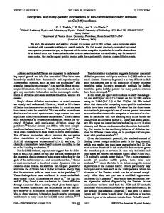
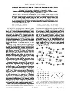
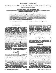
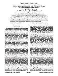
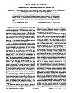
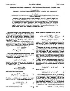
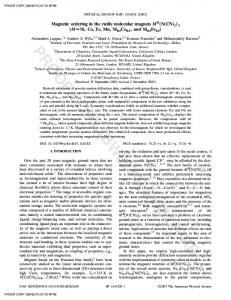
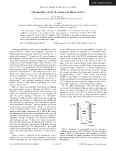
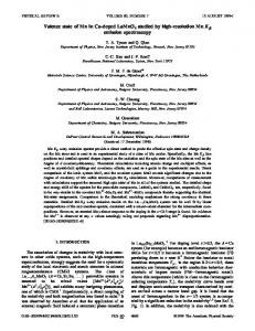
Figure 1 shows the first three conduction and valenceband energy states with m⫽0 obtained for spherical QD’s (T⫽300 K) as a function of the radius. The solid lines correspond to the results of the spherical calculation 共IFBEF兲 and the symbols correspond to the anisotropic calculation 共AFBEF兲. The eigenvalues resulting from the spherical calculation are labeled by the corresponding angular momentum quantum number j and by the parity . The results show that quantum confinement effects becomes stronger in going from PbS to PbSe to PbTe. This is expected since the exciton Bohr radius increases in the same way 关 a 0 (PbS) ⬍a 0 (PbSe)⬍a 0 (PbTe) 兴 . There is almost no discrepancy between the spherical and the anisotropic calculation for the PbS QD’s states. For PbSe, there are appreciable differences only for the excited levels, while for PbTe QD’s this discrepancy is very important even for the ground states. We verified that the convergence of the Y m l j 0 关 n (r/R) 兴 expansions becomes slower for higher anisotropies, higher states and stronger confinement but, yet, the method does converge even for the extreme cases. As an example, considering the lowest radius 共1-nm radius兲 and the highest anisotropy 共PbTe QD兲 studied, the convergence for the first three conduction and valence-band states was achieved for d ⫽200. All the calculation results presented in this paper were done for n⫽l⫽15 (d⫽465). The fundamental transition energies of PbS, PbSe, and PbTe QD’s, calculated by the AFBEF model, are presented in Fig. 2, as functions of the dots radii. The effect of the anisotropy in the energy position of these transitions is shown in Fig. 3, where the difference between the results of the IFBEF and the AFBEF calculation is plotted. For PbS, PbSe, and PbTe, this energy difference is, respectively, about 0.3%, 0.5%, and 4% of the transition energy, for QD radius ranging from 1 to 5 nm. Although for PbS and PbSe the anisotropic contribution to the ground transition is almost
FIG. 1. Energy levels obtained by the IFBEF 共lines兲 and the AFBEF 共symbols兲 calculations as functions of the QD radius. Parts 共a兲, 共b兲, and 共c兲 show the results for PbS, PbSe, and PbTe, respectively.
negligible, it is a significant contribution for PbTe (⌬E ⫽250 meV for 1 nm PbTe QD兲. In order to better understand the role of the anisotropy in the energy spectrum, we play with the PbTe band parameters
PRB 62
EFFECT OF BAND ANISOTROPY ON ELECTRONIC . . .
7361
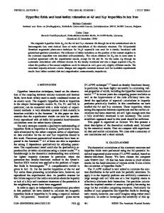
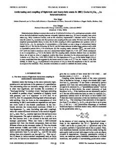
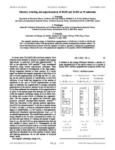
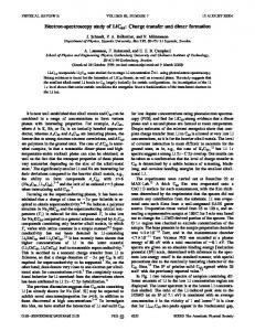
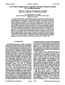
FIG. 4. Transition strengths of a 4-nm PbTe QD assuming different sets of band parameters. From top to bottom the degree of band anisotropy increases: ⫽0,0.25,0.5,0.75, and 1. The dotted and dashed arrows show the energy levels evolve by adding the anisotropy. FIG. 2. Calculated fundamental transitions of PbS 共square兲, PbSe 共circle兲, and PbTe 共triangle兲 QD’s. The dotted lines are guide for the eyes.
starting from the isotropic case 关as defined in Eq. 共10兲兴 and going to the true material parameters shown in Table I. Figure 4 shows the transition energies and oscillator strengths for a 4-nm PbTe QD using a different set of parameters. The top graph shows the isotropic result and the bottom one the result using the true parameters. In between, the used parameters correspond to a linear interpolation between the spherical and true parameters, such as 关 p⫽ p sph⫹(p true⫺ p sph) 兴 where p stands for all band parameters. is a measure of the amount of anisotropy. From top to bottom it varies from 0 to 1 in steps of 0.25. One sees that by increasing the anisotropy () the position of the transitions change significantly and so does the oscillator strengths. The transitions spread out in the energy spectrum and the oscillator strengths are redistributed. Figure 5 shows the AFBEF calculation of the energy spectra of the lead salt QD’s (R⫽4 nm) with all the al-
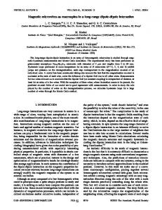
FIG. 3. Energy difference between the IFBEF and AFBEF calculations of the ground-state energy for PbS 共square兲, PbSe 共circle兲, and PbTe 共triangle兲 as a function of the QD radius.
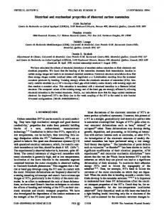
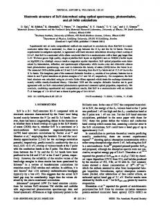
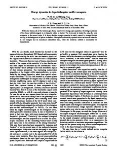
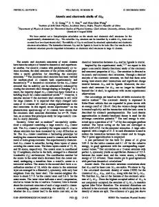
lowed transitions (⌬m⫽0) and the corresponding oscillator strengths. Parts a, b, and c refer to PbS, PbSe, and PbTe, respectively. For comparison, also presented in the same figure are the analogous results using the IFBEF model 共top graphs兲. As explained in the previous section, the transitions strengths between states with different quantum number m are negligible. The obtained results show that for PbS, the spherical approximation and the complete calculation give similar energy spectra up to 1.5 eV. For higher-energy levels however the two calculations show different results. For PbSe and PbTe, in which the band anisotropy is more important, strong differences between the two calculations appear for much lower-energy levels. They are already significant for the first excited state in PbSe while for PbTe the difference is already important for the ground state. The technique presented here 共AFBEF calculation兲 can
FIG. 5. Transition strengths of PbS 共a兲, PbSe 共b兲, and PbTe 共c兲 QD’s with 4-nm radius. The isotropic 共anisotropic兲 results correspond to the top 共bottom兲 graphs.
7362
G. E. TUDURY et al.
also be applied in the case of QD’s with nonspherical shape. The mathematical difficulty of dealing with boundary condition in an ellipsoidal surface is overcome by rescaling the coordinate axes such that the ellipsoid is transformed in a sphere in the new coordinate system. The simplest case would be an ellipsoid of revolution. For example, starting from an oblate or prolate ellipsoidal z-oriented QD, we elongate or contract the z axis 共the new axis z ⬘ ⫽z/a, a is a scale factor兲, transforming the ellipsoidal QD in a spherical one in the new axes x,y,z ⬘ . This means that the k z ⫽⫺iប( / z) operator must be replaced by k z ⫽k z⬘ /a in Eq. 共2兲. By defin-
2 ⫾ ⬘ ing the longitudinal band parameters such as m ⫾ l ⫽a m l and V ⬘l ⫽V l /a, the Hamiltonian remains the same and the mathematical problem of the ellipsoidal QD is reduced to the problem of a spherical QD with renormalized band parameters. For instance, if one starts with an isotropic material in ⫾ kជ space, m ⫾ l ⫽m t and V l ⫽V t , with an ellipsoidal shape where the longitudinal axis (z axis兲 is 10% longer than the transverse ones, this would be mathematically equivalent to the problem of a spherical boundary condition with the parameters m l⬘ ⫽1.21m t and V l⬘ ⫽0.91V t . In this case the anisotropy in real space was transformed into an anisotropy in the reciprocal space. Analogously, an elongation of 20% is equivalent to m ⬘l ⫽1.44m t and V ⬘l ⫽0.83V t . We would like to point out that the resulting anisotropy showed by the renormalized parameters is weaker than the anisotropy of the true lead-salt material 共Table I兲, that is, (m t /m l ) ⫺ ⫽1.96, (m t /m l ) ⫹ ⫽1.36, V l /V t ⫽0.73 in PbS and (m l /m t ) ⫺ ⫽9.7, (m l /m t ) ⫹ ⫽14.3, V l /V t ⫽0.30 in PbTe.
IV. CONCLUSIONS
We have calculated the energy spectrum of lead-salt spherical QD’s using a kជ • pជ formalism. The anisotropic fourband envelope-function model presented here accounts fully for the bands anisotropy, which allowed us to calculate, the electronic structure of PbTe QD’s. The effects of the anisotropy in the transition energies and strengths were systematically investigated, simply by changing the degree of anisotropy in the band parameters. Our results show that for PbS QD’s, where the band parameters are almost isotropic, the complete calculation is only important if one is interested in high-excited states. For PbSe and PbTe QD’s however the effects of the band anisotropy both in the transition positions and strengths are very pronounced, especially for the excited states, and they increase with the confinement. The complete 共anisotropic兲 calculation is thus necessary to obtain the energy spectra of these materials. Furthermore, we have shown that the same technique can be applied to an ellipsoidal QD by rescaling the coordinate axes and transforming the QD in a spherical one, with renormalized band parameters.
PRB 62
APPENDIX A: MIXING OF THE FOUR L POINTS
We assume that the dot eigenfunctions have the form
共 kជ ,rជ 兲 ⫽ 兺 exp共 ⫺l 2 /X 2 兲 exp共 ikជ • ជl 兲 共 rជ ⫺ ជl 兲 , ជl
where the are Wannier functions that can be constructed with small enough width,31 and kជ means each of the wave vectors of the four points L. The parameter X controls how extensive in space is the function and is related to the radius of the dot. When X tends to infinity these wave functions tend to become Bloch waves. With the four wave functions we construct a 4⫻4 secular matrix of H⫺E, where H is the one-electron Hamiltonian for the perfect crystal made out of the dot material. Among the eigenvalues, three are degenerate and the fourth is a singlet. The energy difference between the triplet and the singlet is ⌬E⫽4
N 0 ⫺S (110) N1 S (110) 1 0 共 N 0 ⫹3N 1 兲共 N 0 ⫺N 1 兲
⫹4
V 110
S (200) N 0 ⫺S (200) N1 1 0 共 N 0 ⫹3N 1 兲共 N 0 ⫺N 1 兲
V 200⫹•••
共A1兲
the sum extending over the many shells of neighbors (110), (200), (211), . . . . The many symbols are the following: N 0 ⫽ 具 共 kជ 兲 兩 共 kជ 兲 典 ⫽
兺ជl exp共 ⫺2l 2 /X 2 兲 ,
共A2兲
which is effectively the number of cells inside the dot, N 1 ⫽ 具 共 kជ 兲 兩 共 kជ ⬘ 兲 典 ⫽
兺ជl exp共 ⫺2l 2 /X 2 兲 exp关 i ជl • 共 kជ ⬘ ⫺kជ 兲兴
for different L point vectors kជ and kជ ⬘ . Further, letting nជ mean the vectors of a shell of neighbors such as the shell of vectors a/2(110), a/2(101), . . . , or the shell a/2(200), . . . , we have ជ
S n0 ⫽
exp共 ⫺l 2 /X 2 ⫺ 兩 ជl ⫹nជ 兩 2 /X 2 兲 exp共 ⫺ikជ •nជ 兲 , 兺ជl nជ ,兺 shell ជ
S n1 ⫽
exp共 ⫺l 2 /X 2 ⫺ 兩 ជl ⫹nជ 兩 2 /X 2 兲 兺ជl nជ ,兺 shell ⫻exp共 ⫺ikជ •nជ 兲 exp关 i ជl • 共 kជ⬘ ⫺kជ 兲兴 ,
where the last definition refers to L points with different wave vectors kជ . The energy parameters V nជ are the matrix elements of the Wannier functions V nជ ⫽ 具 共 rជ 兲 兩 H 兩 共 rជ ⫺nជ 兲 典
ACKNOWLEDGMENTS
This work was supported by Conselho Nacional de Desenvolvimento Cientı´fico e Tecnolo´gico–CNPq 共PRONEX兲. G.E.T. and M.V.M. acknowledge support from FAPESP and CNPq 共PRONEX兲, Brazilian agencies.
and determine the energy-band functions of the periodic crystal E 共 kជ 兲 ⫽H 0 ⫹
兺nជ V nជ e ikជ •nជ .
PRB 62
EFFECT OF BAND ANISOTROPY ON ELECTRONIC . . .
冕
TABLE II. Factors determining L point mixing. &R a
N 0 ⫺S (200) N1 S(200) 1 0
4 共 N 0 ⫹3N 1 兲共 N 0 ⫺N 1 兲 ⫺8
10.317 9.251 8.261 5.004 4.353 2.309 1.290 1.033
4
S (220) N 0 ⫺S (220) N1 1 0
1
0
t 2 f 共 n,t 兲
⫺2.676⫻10 ⫺1.518⫻10⫺6 ⫺5.313⫻10⫺6 ⫺5.512⫻10⫺4 ⫺1.530⫻10⫺3 ⫺5.118⫻10⫺2 ⫺3.607⫻10⫺1 ⫺5.887⫻10⫺1
1 ⫺ 2 p 2 ␦ n,p , 2
冕
1
0
t 2 f 共 n,t 兲
1 t f 共 n,t 兲 f 共 p,t 兲 dt⫽ ␦ m,n , 2 2
冕
1
0
t 2 f 共 n,t 兲
sin共 n t 兲 ; t
n and p are integers and t⫽r/R.
1
For a review see, for instance, A.D. Yoffe, Adv. Phys. 42, 173 共1993兲, and references therein. 2 M.G. Burt, U.S. Patent No. 5881200, 1999. 3 Y. Wang, A. Suna, W. Mahler, and R. Kasowski, J. Chem. Phys. 87, 7315 共1987兲. 4 N.F. Borrelli and D.W. Smith, J. Non-Cryst. Solids 180, 25 共1994兲. 5 V.C.S. Reynoso, A.M. de Paula, R.F. Cuevas, J.A. Medeiros Neto, O.L. Alves, C.L. Cesar, and L.C. Barbosa, Electron. Lett. 31, 1013 共1995兲. 6 I. Kang and F.W. Wise, J. Opt. Soc. Am. B 14, 1632 共1997兲. 7 A. Lipovskii, E. Kolobkova, V. Petrikov, I. Kang, A. Olkhovets, T. Krauss, M. Thomas, J. Silcox, F. Wise, Q. Shen, and S. Kycia, Appl. Phys. Lett. 71, 3406 共1997兲. 8 E.R. Thoen, G. Steinmeyer, P. Langlois, E.P. Ippen, G.E. Tudury,
1 d f 共 p,t 兲 1 dt⫽⫺ nSi 关 共 n⫹p 兲兴 t dt 2
1 t
f 共 p,t 兲 dt⫽⫹ 2 ⫺
共 n⫹ p 兲 Si 关 共 n⫹p 兲兴 2 共 n⫺ p 兲 Si 关 共 n⫺p 兲兴 , 2 共B4兲
冕
1
0
t 2 f 共 n,t 兲
d f 共 p,t 兲 1 dt⫽⫺ Ci 共 n ⫺ p 兲 dt 2 1 1 ⫹ Ci 共 n ⫹ p 兲 ⫺ ln共 n⫹p 兲 2 2 1 ⫹ ln共 n⫺ p 兲 2
⫹
共B1兲
where
共B2兲
1 ⫺ nSi 关 共 p⫺n 兲兴 , 共B3兲 2
The solutions of the radial integrals that appear in the calculation are presented below:
f 共 n,t 兲 ⫽
dt⫽ nSi 关 共 n⫹ p 兲兴 ⫹ nSi 关 共 p⫺n 兲兴
APPENDIX B: RADIAL INTEGRALS
0
dt 2
共 N 0 ⫹3N 1 兲共 N 0 ⫺N 1 兲
Therefore, the energy parameters V nជ are related to the bandwidth. Typically, for bandwidths in the order of 10 eV Ref. 32 the energy parameters V are in the order of 0.5 eV. Therefore we can make a crude estimate of the splitting ⌬E using this value for the V’s and calculating the multipliers 共Table II兲 as functions of the effective radius R, given by 4 R 3 /3⫽a 3 N 0 /4. The first nonzero multiplier belongs to the shell (200). The lattice parameter of PbTe is a⫽6.462 Å.33 For a dot radius of R⫽1.0 nm ( 冑2R/a⫽2.2), and V nជ ⯝0.5 eV we obtain ⌬E⯝30 meV, and falls by a factor of 100 when the radius doubled to 2 nm. Further, with increasing R, ⌬E falls off exponentially and becomes increasingly negligible.
冕
d 2 f 共 p,t 兲
⫺8
6.031⫻10 5.549⫻10⫺7 1.375⫻10⫺6 1.693⫻10⫺4 4.797⫻10⫺4 1.811⫻10⫺2 1.525⫻10⫺1 2.739⫻10⫺1
1
7363
再
2n p n 2⫺ p 2 0
if if
n⫹p⫽odd n⫹p⫽even, 共B5兲
冕
1
0
t 2 f 共 n,t 兲
1 1 1 f 共 p,t 兲 dt⫽ Ci 共 n ⫺ p 兲 ⫺ Ci 共 n ⫹p 兲 t 2 2 1 1 ⫹ ln共 n⫹ p 兲 ⫺ ln共 n⫺p 兲 2 2
共B6兲
C.H. Brito Cruz, L.C. Barbosa, and C.L. Cesar, Appl. Phys. Lett. 73, 2149 共1998兲. 9 P.C. Sercel and K.J. Vahala, Phys. Rev. B 42, 3690 共1990兲. 10 K.J. Vahala and P.C. Sercel, Phys. Rev. Lett. 65, 239 共1990兲. 11 L.W. Wang and A. Zunger, J. Chem. Phys. 100, 2394 共1994兲. 12 H. Fu, L.W. Wang, and A. Zunger, Phys. Rev. B 57, 9971 共1998兲. 13 P.E. Lippens and M. Lannoo, Phys. Rev. B 39, 10 935 共1989兲. 14 P.E. Lippens and M. Lannoo, Phys. Rev. B 41, 6079 共1990兲. 15 B. Zorman, M.V. Ramakrishna, and R.A. Friesner, J. Phys. Chem. 99, 7649 共1995兲. 16 R.S. Kane, R.E. Cohen, and R. Silbey, J. Phys. Chem. 100, 7928 共1996兲. 17 A.I. Ekimov, F. Hache, M.C. Schanne-Klein, D. Ricard, C. Flytzanis, I.A. Kudryavtsev, T.V. Yazeva, A.V. Rodina, and Al.L. Efros, J. Opt. Soc. Am. B 10, 100 共1993兲.
7364 18
G. E. TUDURY et al.
D.J. Norris, A. Sacra, C.B. Murray, and M.G. Bawendi, Phys. Rev. Lett. 72, 2612 共1994兲. 19 D.J. Norris and M.G. Bawendi, Phys. Rev. B 53, 16 338 共1996兲. 20 L.E. Brus, Al.L. Efros, and T. Itoh, J. Lumin. 70, 1 共1996兲. 21 C.R.M. de Oliveira, A.M. de Paula, F.O. Plentz Filho, J.A. Medereiros Neto, L.C. Barbosa, O.L. Alves, E.A. Menezes, J.M.M. Rios, H.L. Fragnito, C.H. Brito Cruz, and C.L. Cesar, Appl. Phys. Lett. 66, 439 共1995兲. 22 G. Bastard, Wave Mechanics Applied to Semiconductor Heterostructures 共Wiley, New York, 1991兲. 23 D.L. Mitchell and R.F. Wallis, Phys. Rev. 151, 581 共1966兲. 24 J.O. Dimmock, in The Physics of Semimetals and Narrow-Gap Semiconductors, edited by D.L. Carter and R.T. Bates 共Pergamon, Oxford, 1971兲. 25 R. Dalven, in Solid State Physics: Advances in Research and Applications, edited by F. Seitz, D. Turnbull, and H. Ehrenreich 共Academic, New York, 1973兲, Vol. 28, p. 179.
PRB 62
The use of these radial functions over the set j l (k ln r) 关with j l (k ln R)⫽0兴 makes the calculation very convenient once they do not depend on l and lead to a fast converging sine Fourier series. Furthermore, the resulting radial integrals used in both, the energy levels and oscillator strengths calculation, are easily performed, as shown in Appendix B. 27 W.H. Press, S.A. Teukolsky, W.T. Vetterling, and B.P. Flannery, Numerical Recipes in Fortran 共Cambridge University Press, Cambridge, 1992兲. 28 M.E. Rose, Elementary Theory of Angular Momentum 共Wiley, New York, 1957兲. 29 H. Preier, Appl. Phys. 20, 189 共1979兲. 30 C.R. Hewes, M.S. Adler, and S.D. Senturia, Phys. Rev. B 7, 5195 共1973兲. 31 L.G. Ferreira and N.J. Parada, J. Phys. C 4, 15 共1971兲. 32 S.-H. Wei and A. Zunger, Phys. Rev. B 55, 13 605 共1997兲. 33 R. Dalven, Infrared Phys. 9, 141 共1969兲. 26