Variational Gaussian Approximation for Poisson Data Simon R. Arridge∗
Kazufumi Ito†
Bangti Jin∗
Chen Zhang∗
arXiv:1709.05885v1 [math.NA] 18 Sep 2017
Abstract The Poisson model is frequently employed to describe count data, but in a Bayesian context it leads to an analytically intractable posterior probability distribution. In this work, we analyze a variational Gaussian approximation to the posterior distribution arising from the Poisson model with a Gaussian prior. This is achieved by seeking an optimal Gaussian distribution minimizing the Kullback-Leibler divergence from the posterior distribution to the approximation, or equivalently maximizing the lower bound for the model evidence. We derive an explicit expression for the lower bound, and show the existence and uniqueness of the optimal Gaussian approximation. The lower bound functional can be viewed as a variant of classical Tikhonov regularization that penalizes also the covariance. Then we develop an efficient alternating direction maximization algorithm for solving the optimization problem, and analyze its convergence. We discuss strategies for reducing the computational complexity via low rank structure of the forward operator and the sparsity of the covariance. Further, as an application of the lower bound, we discuss hierarchical Bayesian modeling for selecting the hyperparameter in the prior distribution, and propose a monotonically convergent algorithm for determining the hyperparameter. We present extensive numerical experiments to illustrate the Gaussian approximation and the algorithms. Keywords: Poisson data, variational Gaussian approximation, Kullback-Leibler divergence, alternating direction maximization, hierarchical modeling
1
Introduction
This work is concerned with Gaussian approximations to a Poisson noise model for linear inverse problems. The Poisson model is popular for modeling count data, where the response variable follows a Poisson distribution with a parameter that is the exponential of a linear combination of the unknown parameters. The model is especially suitable for low count data, where the standard Gaussian model is inadequate. It has found many successful practical applications, including transmission tomography [41, 12]. One traditional approach to parameter estimation with the Poisson model is the maximum likelihood method or penalized variants with a convex penalty. This leads to a convex optimization problem, whose solution is then taken as an approximation to the true solution. This approach has been extensively studied, and we refer interested readers to the survey [18] for a comprehensive account on important developments along this line. However, this approach gives only a point estimator, and does not allow quantifying the associated uncertainties directly. In this work, we aim at a full Bayesian treatment of the problem, where both the point estimator (mean) and the associated uncertainties (covariance) are of interest [23, 38]. We shall focus on the case of a Gaussian prior, which forms the basis of many other important priors, e.g., sparsity prior via scale mixture representation. Then following the Bayesian procedure, we arrive at a posterior probability distribution, which however is analytically intractable due to the nonstandard form of the likelihood function for the Poisson model. We will explain this more precisely in Section 2. To explore the posterior state space, instead of applying popular general-purposed sampling techniques, e.g., Markov chain Monte Carlo (MCMC), we employ a variational Gaussian approximation (VGA). The VGA is one extremely popular approximate inference technique in machine learning [40, 8]. ∗ Department of Computer Science, University College London, Gower Street, London WC1E 6BT, UK (s.r.arridge,b.jin,
[email protected]) † Department of Mathematics, North Carolina State University, Raleigh, NC 27607, USA (
[email protected])
1
Specifically, we seek an optimal Gaussian approximation to the non-Gaussian posterior distribution with respect to the Kullback-Leibler divergence. The approach leads to a large-scale optimization problem over the mean x ¯ and covariance C (of the Gaussian approximation). In practice, it generally delivers an accurate approximation in an efficient manner, and thus has received immense attention in recent years in many different areas [17, 3, 8, 2]. By its very construction, it also gives a lower bound to the model evidence, which facilitates its use in model selection. However, a systematic theoretical understanding of the approach remains largely missing. In this work, we shall study the analytical properties and develop an efficient algorithm for the VGA in the context of Poisson data (with the log linear link function). We shall provide a detailed analysis of the resulting optimization problem. The study sheds interesting new insights into the approach from the perspective of regularization. Our main contributions are as follows. First, we derive explicit expressions for the objective functional and its gradient, and establish its strict concavity and the well-posedness of the optimization problem. Second, we develop an efficient numerical algorithm for finding the optimal Gaussian approximation, and discuss its convergence properties. The algorithm is of alternating maximization (coordinate ascent) nature, and it updates the mean x ¯ and covariance C alternatingly by a globally convergent Newton method and a fixed point iteration, respectively. We also discuss strategies for its efficient implementation, by leveraging realistic structure of inverse problems, e.g., low-rank nature of the forward map A and sparsity of the covariance C, to reduce the computational complexity. Third, we illustrate the use of the evidence lower bound for hyperparameter selection within a hierarchical Bayesian framework, leading to a purely data-driven approach for determining the regularization parameter, whose proper choice is notoriously challenging. We shall develop a monotonically convergent algorithm for determining the hyperparameter in the Gaussian prior. Last, we illustrate the approach and the algorithms with extensive numerical experiments for one- and two-dimensional examples. Last, we discuss existing works on Poisson models. The majority of existing works aim at recovering point estimators, either iteratively or by a variational framework [18]. Recently, Bardsley and Luttman [4] described a Metroplis-Hastings algorithm for exploring the posterior distribution (with rectified linear inverse link function), where the proposal samples are drawn from the Laplace approximation (cf. Remark 3.1). The Poisson model (2.2) belongs to generalized linear models (GLMs), to which the VGA has been applied in statistics and machine learning [32, 26, 8, 36]. Ormerod and Wand [32] suggested a variational approximation strategy for fitting GLMs suitable for grouped data. Challis and Barber [8] systematically studied VGA for GLMs and various extensions. The focus of these interesting works [32, 26, 8, 36] is on the development of the general VGA methodology and its applications to concrete problems, and do not study analytical properties and computational techniques for the lower bound functional, which is the main goal of this work. The rest of the paper is organized as follows. In Section 2, we describe the Poisson model, and formulate the posterior probability distribution. Then in Section 3, we develop the variational Gaussian approximation, and analyze its basic analytical properties. In Section 4, we propose an efficient numerical algorithm for finding the optimal Gaussian approximation, and in Section 5, we apply the lower bound to hyperparameter selection within a hierarchical Bayesian framework. In Section 6 we present numerical results for several examples. In two appendices, we provide further discussions on the convergence of the fixed point iteration (4.4) and the differentiability of the regularized solution.
2
Notation and problem setting
First we recall some standard notation in linear algebra. Throughout, (real-valued) vectors and matrices are denoted by bold lower- and upper-case letters, respectively, and the vectors are always column vectors. We will use the notation (·, ·) to denote the usual Euclidean inner product. We shall slightly abuse the notation (·, ·) also for the inner product for matrices. That is, for two matrices X, Y ∈ Rn×m , we define (X, Y) = tr(XYt ) = tr(Xt Y),
2
where tr(·) denotes taking the trace of a square matrix, and the superscript t denotes the transpose of a vector or matrix. This inner product induces the usual Frobenius norm for matrices. We shall use extensively the cyclic property of the trace operator tr(·): for three matrices X, Y, Z of appropriate size, there holds tr(XYZ) = tr(YZX) = tr(ZXY). We shall also use the notation diag(·) for a vector and a square matrix, which gives a diagonal matrix and a column vector from the diagonals of the matrix, respectively, in the same manner as the diag function in MATLAB. The notation N = {0, 1, . . .} denotes the set of natural numbers. Further, the notation ◦ + denotes the Hadamard product of two matrices or vectors. Last, we denote by Sm ⊂ Rm×m the set of m×m m×m symmetric positive definite matrices in R , Im the identity matrix in R , and by | · | and k · k the determinant and the spectral norm, respectively, of a square matrix. Throughout, we view exponential, logarithm and factorial of a vector as componentwise operation. Next we recall the finite-dimensional Poisson data model. Let x ∈ Rm be the unknown signal, ai ∈ Rm , i = 1, . . . , n, and y ∈ Nn ⊂ Rn be the data vector. We stack the column vectors ai into a matrix A by A = [ati ] ∈ Rn×m . Given the matrix A and data y ∈ Nn , the Poisson model takes the form: yi ∼ Pois(e(ai ,x) ),
i = 1, 2, . . . , n.
Thus, the likelihood function p(yi |x) for the data point yi is given by p(yi |x) =
λyi i e−λi , yi !
λi = e(ai ,x) , i = 1, . . . , n.
(2.1)
It is worth noting that the exponential function enters into the Poisson parameter λ. This is commonly known as the log link function or log-linear model in the statistical literature [7]. There are several other models for the (inverse) link functions, e.g., rectified-linear and softplus [33], each having its own pros and cons for modeling count data. In this work, we shall focus on the log link function. Also this model can be viewed as a simplified statistical model for transmission tomography [41, 12]. The likelihood function p(yi |x) can be equivalently written as p(yi |x) = eyi (ai ,x)−e
(ai ,x) −ln(yi !)
.
Under the independent identically distributed (i.i.d.) assumption on the data points yi , the likelihood function p(y|x) of the data vector y is given by p(y|x) =
n Y
p(yi |x) = e(Ax,y)−(e
Ax
,1n )−(ln(y!),1n )
,
(2.2)
i=1
where 1n ∈ Rn is the vector with all entries equal to unity, i.e., 1n = [1, . . . , 1]t ∈ Rn . Further, we assume that the unknown x follows a Gaussian prior p(x), i.e., m
1
1
t
p(x) = N (x; µ0 , C0 ) := (2π)− 2 |C0 |− 2 e− 2 (x−µ0 )
C−1 0 (x−µ0 )
,
+ where µ0 ∈ Rm and C0 ∈ Sm denote the mean and covariance of the Gaussian prior, respectively, and N denotes the normal distribution. In the framework of variational regularization, the corresponding penalty 12 (x − µ0 )t C−1 0 (x − µ0 ) often imposes certain smoothness constraint. The Gaussian prior p(x) may depend on additional hyperparameters, cf. Section 5 for details. Then by Bayes’ formula, the posterior probability distribution p(x|y) is given by
p(x|y) = Z −1 p(x, y),
(2.3)
where the joint distribution p(x, y) is defined by m
1
p(x, y) = (2π)− 2 |C0 |− 2 e(Ax,y)−(e
Ax
3
,1n )−(ln(y!),1n )− 12 (x−µ0 )t C−1 0 (x−µ0 )
,
and the normalizing constant Z(y), which depends only on the given data y, is given by Z Z(y) = p(y) = p(x, y)dx. That is, the normalizing constant Z is an integral living in a very high-dimensional space if the parameter dimension m is large. Thus it is computationally intractable, and so is the posterior distribution p(x|y), since it also involves the constant Z. The quantity Z is commonly known as model evidence in the literature, and it underlies many model selection rules, e.g., Bayes factor [24]. Thus the reliable approximation of Z(y) is important in certain tasks. The posterior distribution p(x|y) given in (2.3) is the Bayesian solution to the Poisson model (2.1) (under a Gaussian prior), and it contains all the information about the inverse problem. In order to explore the posterior state space, one typically employs Markov chain Monte Carlo methods, which, however, can be prohibitively expensive for high-dimensional problems, apart from the well-known challenge in diagnosing the convergence of the Markov chain. To overcome the challenge, over the last two decades, a large number of approximate inference methods have been developed, including mean-field approximation [40], expectation propagation [30] and variational Gaussian approximation (VGA) [31, 8]. In all these approximations, we aim at finding a best approximate yet tractable distribution q(x) within a family of parametric/nonparametric probability distributions, by minimizing the error in a certain probability metric, prominently the Kullback-Leibler divergence DKL (q||p), cf. Section 3.1 below. In this work, we shall employ the VGA to obtain an optimal Gaussian approximation q(x) to the posterior distribution p(x|y) in the Kullback-Leibler divergence DKL (q||p). Fitting a Gaussian to an intractable distribution is a well-established norm for approximate Bayesian inference, and it has demonstrated success in many practical applications [17, 3, 8, 2]. The popularity can be largely attributed to the fact that the Gaussian approximation is computationally attractive, and yet delivers reasonable accuracy for a wide range of problems, due to the good analytical properties and great flexibility of the Gaussian family. However, analytical properties of approximate inference procedures are rarely studied. In the context of Poisson mixed models, the asymptotic normality of the estimator and its convergence rate was analyzed [16]. In a general setting, some theoretical issues were studied in [34, 29].
3
Gaussian variational approximation
In this section, we recall the Kullback-Leibler divergence, derive explicit expressions for the lower bound functional and its gradient, and discuss basic analytic properties, e.g., concavity and existence.
3.1
Kullback-Leibler divergence
The Kullback-Leibler divergence is one of the most popular metrics for measuring the distance between two probability distributions. The Kullback-Leibler (KL) divergence [28] from one probability distribution p to another distribution q is a functional defined by Z q(x) dx. (3.1) DKL (q||p) = q(x)ln p(x) Clearly, KL divergence is not symmetric and thus not a metric R in the mathematical sense. Since the logarithm function ln x is concave and that q is normalized, i.e., q(x)dx = 1, by Jensen’s inequality, we can derive the nonnegativity of the KL divergence: Z Z q(x) p(x) DKL (q||p) = q(x)ln dx = − q(x)ln dx p(x) q(x) (3.2) Z Z p(x) ≥ −ln q(x) dx = −ln p(x)dx = 0. q(x) Further, DKL (q||p) = 0 if and only if p = q almost everywhere. 4
Due to unsymmetry of the KL divergence, to find an approximation q to the target distribution p, there are two options, i.e., minimizing either DKL (q||p) or DKL (p||q). These two options lead to different approximations. It was pointed out in [6, Section 10.1.2] that minimizing DKL (p||q) tends to find the average of modes of p, while minimizing DKL (q||p) tends to find one exact mode. Traditionally, the former is used in expectation propagation, and the latter in variational Bayes. In this work, we focus on the approach min DKL (q||p), which leads to the VGA to be described below. ˆ be Remark 3.1. In practice, the so-called Laplace approximation is quite popular [39]. Specifically, let x ˆ , i.e., x ˆ = arg minx∈Rm g(x), where g(x) = − ln p(x|y) is the maximum a posteriori (MAP) estimator x ˆ: the negative log posterior distribution. Consider the Taylor expansion of g(x) at the MAP estimator x ˆ )t H(x − x ˆ) ˆ ) + 21 (x − x g(x) ≈ g(ˆ x) + (∇g(ˆ x), x − x ˆ )t H(x − x ˆ ), = g(ˆ x) + 21 (x − x since ∇g(ˆ x) vanishes. The Hessian H of g(x) is given by H = At diag(eAˆx )A + C−1 0 . Thus, x ˆ might serve as an approximate posterior mean, and the inverse Hessian H−1 as an approximate posterior covariance. However, unlike the VGA discussed below, it lacks the optimality as evidence lower bound (within the Gaussian family), and thus may be suboptimal for model selection etc.
3.2
Variational Gaussian lower bound
Now we derive the variational Gaussian lower bound. By substituting p(x) with the posterior distribution p(x|y) in (3.1), we obtain Z q(x) dx. DKL (q(x)||p(x|y)) = q(x)ln p(x|y) Since the posterior distribution p(x|y) depends on the unknown normalizing constant Z(y), the integral on the right hand side is not computable. Nonetheless, given y, Z(y) is fixed. In view of the identity Z Z p(x, y) q(x) lnZ = q(x)ln dx + q(x)ln dx, q(x) p(x|y) instead of minimizing DKL (q(x)||p(x|y)), we may equivalently maximize the functional Z p(x, y) F (q, y) = q(x)ln dx. q(x)
(3.3)
By (3.2), we have DKL (q(x)||p(x|y)) ≥ 0, and thus lnZ ≥ F (q, y). That is, F (q, y) provides a lower bound on the model evidence Z, for any choice of the distribution q. For any fixed q, F (q, y) may be used as a substitute for the analytically intractable model evidence Z(y), and hence it is called an evidence lower bound (ELBO). Since the data y is fixed, it will be suppressed from F (q, y) below. In the VGA, we restrict our choice of q to Gaussian distributions. Meanwhile, a Gaussian distribution q(x) is fully + characterized by its mean x ¯ ∈ Rm and covariance C ∈ Sm ⊂ Rm×m , i.e., q(x) = N (x; x ¯, C). + Thus, F (q) is actually a function of x ¯ ∈ Rm and C ∈ Sm , and will be written as F (¯ x, C) below. Then the approach seeks optimal variational parameters (¯ x, C) to maximize ELBO. This step turns a challenging sampling problem into a computationally more tractable optimization problem. The next result gives an explicit expression for the lower bound F (¯ x, C).
5
Proposition 3.1. For any fixed y, µ0 and C0 , the lower bound F (¯ x, C) is given by t
1
x − µ0 )t C−1 F (¯ x, C) = (y, A¯ x) − (1n , eA¯x+ 2 diag(ACA ) ) − 21 (¯ x − µ0 ) − 12 tr(C−1 0 C) 0 (¯ +
1 2
ln |C| −
1 2
ln |C0 | +
m 2
− (1n , ln(y!)).
(3.4)
Proof. By the definition of the functional F (¯ x, C) and the joint distribution p(x, y), we have Z h 1 1 F (¯ x, C) = N (x; x ¯, C) ln|C0 |− 2 − ln|C|− 2 + (Ax, y) − (eAx , 1n ) − (ln(y!), 1n ) i t −1 1 − 21 (x − µ0 )t C−1 (x − x ¯ ) C (x − x ¯ ) dx. (x − µ ) + 0 0 2 R It suffices to evaluate the integrals termwise. Clearly, we have N (x; x ¯, C)(Ax, y)dx = (A¯ x, y). Next, using moment generating function, we have Z XZ Ax N (x; x ¯, C)(e , 1n )dx = N (x; x ¯, C)e(ai ,x) dx i
=
X
1
t
1
t
e(ai ,¯x)+ 2 ai Cai = (1n , eA¯x+ 2 diag(ACA ) ).
i
With the Cholesky decomposition C = LLt , for z ∼ N (0, Im ), x = µ + Lz ∼ N (x; µ, C). This and the bias-variance decomposition yield (Eq(x) [·] takes expectation with respect to the density q(x)) Eq(x) [xt Ax] = EN (z;0,Im ) [(µ + Lz)t A(µ + Lz)] = µt Aµ + EN (z;0,Im ) [zt Lt ALz]. By the cyclic property of trace, we have EN (z;0,Im ) [zt Lt ALz] = tr(Lt AL) = tr(ALLt ) = tr(AC). In particular, this gives Eq(x) [(x − µ0 )t C−1 x − µ0 )t C−1 x − µ0 ) + tr(C−1 0 (x − µ0 )] = (¯ 0 (¯ 0 C), and Eq(x) [(x − x ¯)t C−1 (x − x ¯)] = m. Collecting preceding identities completes the proof of the proposition. Remark 3.2. The terms in the functional F (¯ x, C) in (3.4) admit interesting interpretation in the lens of classical Tikhonov regularization (see, e.g., [11, 19, 37]). To this end, it is instructive to rewrite it as t
1
F (¯ x, C) =(y, A¯ x) − (1n , eA¯x+ 2 diag(ACA ) ) − (1n , ln(y!)) − 21 (¯ x − µ0 )t C−1 x − µ0 ) 0 (¯ − 21 tr(C−1 0 C) +
1 2
ln |C| −
1 2
ln |C0 | +
m 2.
The first line represents the fidelity or “pseudo-likelihood” function. It is worth noting that it actually involves the covariance C. In the absence of the covariance C, it recovers the familiar log likelihood for Poisson data, cf. Remark 3.1. The second line imposes a quadratic penalty on the mean x ¯. This term recovers the familiar penalty in Tikhonov regularization (except that it is imposed on x ¯). Recall that the + function − ln |C| is strictly convex in C ∈ Sm [13, Lemma 6.2.2]. Thus, one may define the corresponding Bregman divergence d(C, C0 ). In view of the identities [9] ∂ −1 tr(CC−1 0 ) = C0 ∂C
and
∂ ln |C| = C−1 . ∂C
simple computation gives the following expression for the divergence: −1 d(C, C0 ) = tr(C−1 0 C) − ln |C0 C| − m ≥ 0.
6
(3.5)
Statistically, it is the Kullback-Leibler divergence between two Gaussians of identical mean. The divergence d(C, C0 ) provides a distance measure between the prior covariance C0 and the posterior one C. Let {(λi , vi )}m i=1 be the pairs of generalized eigenvalues and eigenfunctions of the pencil (C, C0 ), i.e., Cvi = λi C0 vi . Then it can be expressed as d(C, C0 ) =
m X
(λi − ln λi − 1).
i=1
This identity directly indicates that d(C, C0 ) ≤ c implies kCk ≤ c and kC−1 k ≤ c, where here and below c denotes a generic constant which may change at each occurrence. Thus, the third line regularizes the posterior covariance C by requesting nearness to the prior one C0 in Bregman divergence. It is interesting to observe that the Gaussian prior implicitly induces a penalty on C, although it is not directly enforced. In statistics, the Bregman divergence d(C, C0 ) is also known as Stein’s loss [21]. In recent years, the Bregman divergence d(C, C0 ) has been employed in clustering, graphical models, sparse covariance estimate and low-rank matrix recovery etc. [27, 35].
3.3
Theoretical properties of the lower bound
Now we study basic analytical properties, i.e., concavity, existence and uniqueness of maximizer, and gradient of the functional F (¯ x, C) defined in (3.4), from the perspective of optimization. A first result shows the concavity of F (¯ x, C). Let X and Y be two convex sets. Recall that a functional f : X × Y → R is said to be jointly concave, if and only if f (λx1 + (1 − λ)x2 , λy1 + (1 − λ)y2 ) ≥ λf (x1 , y1 ) + (1 − λ)f (x2 , y2 ) for all x1 , x2 ∈ X, y1 , y2 ∈ Y and λ ∈ [0, 1]. Further, f is called strictly jointly concave if the inequality + is strict for any (x1 , y1 ) 6= (x1 , y1 ) and λ ∈ (0, 1). It is easy to see that Sm is a convex set. + , the functional F (¯ x, C) is strictly jointly concave with respect to x ¯ ∈ Rm Theorem 3.1. For any C0 ∈ Sm + and C ∈ Sm .
Proof. It suffices to consider the terms apart from the linear terms (y, A¯ x) and − 21 tr(C−1 0 C) and the 1 m 1 t constant term − 2 ln|C0 | + 2 − (1n , ln(y!)). Since A¯ x + 2 diag(ACA ) is linear in x ¯ and C, and ext 1 ponentiation preserves convexity, the term −(1n , eA¯x+ 2 diag(ACA ) ) is also jointly concave. Next, the 1 t −1 + . Last, the log-determinant ln |C| term − 2 (¯ x − µ0 ) C0 (¯ x − µ0 ) is strictly concave for any C0 ∈ Sm + is strictly concave over Sm [13, Lemma 6.2.2]. The assertion follows since strict concavity is preserved under summation. Next, we show the well-posedness of the optimization problem in VGA. Theorem 3.2. There exists a unique pair of (¯ x, C) solving the optimization problem max
+ x ¯∈Rm ,C∈Sm
F (¯ x, C)
(3.6)
Proof. The proof follows by direct methods in calculus of variation, and we only briefly sketch it. Clearly, + there exists a maximizing sequence, denoted by {(¯ xk , Ck )} ⊂ Rm × Sm , and we may assume F (¯ xk , Ck ) ≥ c =: F (µ0 , C0 ). Thus, by (3.4) in Proposition 3.1 and the divergence d(C, C0 ), we have k
(A¯ xk , y) − (¯ xk − µ0 )t C−1 xk − µ0 ) − d(Ck , C0 ) ≥ c + (eA¯x 0 (¯
+ 21 diag(ACk At )
, 1n ) ≥ c.
By the Cauchy-Schwarz inequality, we have (¯ xk − µ0 )t C−1 xk − µ0 ) + d(Ck , C0 ) ≤ c. This immediately 0 (¯ k k k −1 implies a uniform bound on {(¯ x , C )} and {(C ) }. Thus, there exists a convergent subsequence, + relabeled as {(¯ xk , Ck )}, with a limit (¯ x ∗ , C ∗ ) ∈ Rm × S m . Then by the continuity of the functional F ∗ ∗ in (¯ x, C), we deduce that (¯ x , C ) is a maximizer to F (¯ x, C), i.e., the existence of a maximizer. The uniqueness follows from the strict joint-concavity of F (¯ x, C), cf. Theorem 3.1. 7
Since F is composed of smooth functions, clearly it is smooth. Next we give the gradient formulae, which are useful for developing numerical algorithms below. Theorem 3.3. The gradients of the functional F (¯ x, C) with respect to x ¯ and C are respectively given by t 1 ∂F = At y − At eA¯x+ 2 diag(ACA ) − C−1 x − µ0 ), 0 (¯ ∂¯ x t 1 ∂F −1 = 12 [−At diag(eA¯x+ 2 diag(ACA ) )A − C−1 ]. 0 +C ∂C
Proof. Let d = A¯ x + 21 diag(ACAt ). Then by the chain rule n n n X ∂ ∂ X dj X ∂edj ∂dj (1n , ed ) = = e = edj (A)ji . ∂x ¯i ∂x ¯i j=1 ∂d ∂ x ¯ j i j=1 j=1 ∂ d t d That is, we have ∂¯ x (1n , e ) = A e , showing the first formula. Next we derive the gradient with respect t 1 to the covariance C. In view of (3.5), it remains to differentiate the term (1n , eA¯x+ 2 diag(ACA ) ) with respect to C. To this end, let H be a small perturbation to C. By Taylor expansion, and with the t 1 diagonal matrix D = diag(eA¯x+ 2 diag(ACA ) ), we deduce 1
t
t
1
(1n , eA¯x+ 2 diag(A(C+H)A ) ) − (1n , eA¯x+ 2 diag(ACA ) ) = (D, 12 diag(AHAt )) + O(kHk2 ). Since the matrix D is diagonal, by the cyclic property of trace, we have (D, 21 diag(AHAt )) = (D, 12 (AHAt )) = 21 tr(DAHt At ) = 12 tr(At DAHt ) = 12 (At DA, H). Now the definition of the gradient completes the proof. An immediate corollary is the following optimality system. Corollary 3.1. The necessary and sufficient optimality system of problem (3.6) is given by t
1
At y − At eA¯x+ 2 diag(ACA ) − C−1 x − µ0 ) = 0, 0 (¯ t
1
C−1 − At diag(eA¯x+ 2 diag(ACA ) )A − C−1 0 = 0. Remark 3.3. Challis and Barber [8] showed that for log-concave site posterior potentials, the variational lower bound is jointly concave in x ¯ and the Cholesky factor L of the covariance C. This assertion holds also for the lower bound F (¯ x, C) in (3.4), i.e., joint concavity with respect to (¯ x, L). Remark 3.4. Corollary 3.1 indicates that the covariance C∗ of the optimal Gaussian approximation q ∗ (x) is of the following form: t (C∗ )−1 = C−1 0 + A DA, for some diagonal matrix D. Thus it is tempting that one may minimize with respect to D instead of C in order to reduce the complexity of the algorithm, by reducing the number of unknowns from m2 to m. However, F is generally not concave with respect to D; see [26] for a one-dimensional counterexample. The loss of concavity might complicate the analysis and computation. Remark 3.5. In practice, the parameter x in the model (2.2) often admits physical constraint. Thus it is natural to impose a box constraint on the mean x ¯ in problem (3.6), e.g., cl ≤ x ¯i ≤ cu , i = 1, . . . , m, for some cl < cu . This can be easily incorporated into the optimality system in Corollary 3.1, and the algorithms below remain valid upon minor changes, e.g., including a pointwise projection operator in the update of x ¯.
8
4
Numerical algorithm and its complexity analysis
Now we develop an efficient numerical algorithm, which is of alternating direction maximization type, provide an analysis of its complexity, and discuss strategies for complexity reduction.
4.1
Numerical algorithm
In view of the strict concavity of F (¯ x, C), it suffices to solve the optimality system (cf. Corollary 3.1): t
1
At y − At eA¯x+ 2 diag(ACA ) − C−1 x − µ0 ) = 0, 0 (¯ C
−1
t
− A diag(e
A¯ x+ 21 diag(ACAt )
)A −
C−1 0
= 0.
(4.1) (4.2)
This consists of a coupled nonlinear system for (¯ x, C). We shall solve the system by alternatingly maximizing F (¯ x, C) with respect to x ¯ and C, i.e., coordinate ascent. From the strict concavity in Theorem 3.1, we deduce that for a fixed C, (4.1) has a unique solution x ¯, and similarly, for a fixed x ¯, (4.2) has a unique solution C. Below, we discuss the efficient numerical solution of (4.1)–(4.2). 4.1.1
Newton method for updating x ¯
To solve x ¯ from (4.1), for a fixed C, we employ a Newton method. Let the nonlinear map G : Rm → Rm be defined by t 1 x − µ0 ) − At y. G(¯ x) = At eA¯x+ 2 diag(ACA ) + C−1 0 (¯ The Jacobian ∂G of the map G is given by t
1
−1 ∂G(¯ x) = At diag(eA¯x+ 2 diag(ACA ) )A + C−1 0 ≥ C0 ,
where the partial ordering ≥ is in the sense of symmetric positive definite matrix, i.e., X ≥ Y if and only if X − Y is positive semidefinite. That is, the Jacobian ∂G(¯ x) is uniformly invertible (since the prior covariance C−1 x, C) in x ¯. 0 is invertible). This concurs with the strict concavity of the functional F (¯ This motivates the use of the Newton method or its variants: for a nonlinear system with uniformly invertible Jacobians, the Newton method converges globally [25]. Specifically, given x ¯0 , we iterate ∂G(¯ xk )δ¯ x = −G(¯ xk ),
x ¯k+1 = x ¯k + δ¯ x.
(4.3)
The main cost of the Newton update (4.3) lies in solving the linear system involving ∂G(¯ xk ). Clearly, the k Jacobian ∂G(¯ x ) is symmetric and positive definite, and thus the (preconditioned) conjugate gradient method is a natural choice for solving the linear system. One may use C−1 0 (or the diagonal part of the Jacobian ∂G(¯ x)) as a preconditioner. It is worth noting that inverting the Jacobian ∂G(¯ x) is identical with one fixed point update of the covariance C below. In the presence of a priori structural information, this can be carried out efficiently even for very large-scale problems; see Section 4.2 below for further details. By the fast local convergence of the Newton method, a few iterations suffice the desired accuracy, which is fully confirmed by our numerical experiments. 4.1.2
Fixed-point method for updating C
Next we turn to the solution of (4.2) for updating C, with x ¯ fixed. There are several different strategies, and we shall describe two of them below. The first option is to employ a Newton method. Let the nonlinear map S : Rm×m → Rm×m be defined by t
t A¯ x+diag(ACA ) S(C) = C−1 − C−1 )A. 0 − A diag(e
The Jacobian ∂S of the map S is given by t
∂S(C)[H] = −C−1 HC−1 − At diag(eA¯x+diag(ACA ) )diag(AHAt )A. 9
It can be verified that the map ∂S(C) is symmetric with a uniformly bounded inverse (see the proof of Theorem B.1 in the appendix for details). However, its explicit form seems not available due to the presence of the operator diag. Nonetheless, one can apply a (preconditioned) conjugate gradient method for updating C. The Newton iteration is guaranteed to converge globally. The second option is to use a fixed-point iteration. This choice is very attractive since it avoids solving huge linear systems. Specifically, given an initial guess C0 , we iterate by 1
Dk = diag(eA¯x+ 2 diag(AC
k
At )
t k −1 Ck+1 = (C−1 . 0 + A D A)
),
(4.4)
Conceptually, it has the flavor of a classical fixed point scheme for solving algebraic Riccati equations in Kalman filtering [1], and it has also been used in a slightly different context of variational inference with Gaussian processes [26]. Numerically, each inner iteration of (4.4) involves computing the vector diag(ACk At ) (which should be regarded as computing ai Ck ati , i = 1, . . . , m, instead of forming the full matrix ACk At ) and a matrix inversion. Next we briefly discuss the convergence of (4.4). Clearly, for all iterates Ck , we have Ck ≤ C0 . We claim λmax (Ck ) ≤ λmax (C0 ). To see this, let v ∈ Rm be a unit eigenvector corresponding to the largest eigenvalue λmax (Ck ), i.e., vt Ck v = λmax (Ck ). Then by the minmax principle λmax (Ck ) = vt Ck v ≤ vt C0 v ≤ sup vt C0 v = λmax (C0 ). v∈Sm
Thus, the sequence {Ck }∞ k=1 generated by the iteration (4.4) is uniformly bounded in the spectral norm (and thus any norm due to the norm equivalence in a finite-dimensional space). Hence, there exists a convergent subsequence, also relabeled as {Ck }, such that Ck → C∗ , for some C∗ . In practice, the iterates converge fairly steadily to the unique solution to (4.2), which however remains to be established. In Appendix A, we show a certain “monotone” type convergence of (4.4) for the initial guess C0 = C0 . 4.1.3
Variational Gaussian approximation algorithm
With the preceding two inner solvers, we are ready to state the complete procedure in Algorithm 1. One natural stopping criterion at Step 7 is to monitor ELBO. However, computing ELBO can be expensive and cheap alternatives, e.g., relative change of the mean x ¯, might be considered. Note that Step 3 of Algorithm 1, i.e., randomized singular value decomposition (rSVD), has to be carried out only once, and it constitutes a preprocessing step. Its crucial role will be discussed in Section 4.2 below. With exact inner updates (¯ xk , Ck ), by the alternating maximizing property, the sequence {F (¯ xk , Ck )} is guaranteed to be monotonically increasing, i.e., F (¯ x0 , C0 ) ≤ F (¯ x1 , C0 ) ≤ F (¯ x1 , C1 ) ≤ ... ≤ F (¯ xk , Ck ) ≤ ..., with the inequality being strict until convergence is reached. Further, F (¯ xk , Ck ) ≤ ln Z(y). Thus, k k {F (¯ x , C )} converges. Further, by [5, Prop. 2.7.1], the coordinate ascent method converges if the maximization with respect to each coordinate is uniquely attained. Clearly, Algorithm 1 is a coordinate ascent method for F (¯ x, C), and F (¯ x, C) satisfies the unique solvability condition. Thus the sequence {(¯ xk , Ck )} generated by Algorithm 1 converges to the unique maximizer of F (¯ x, C).
4.2
Complexity analysis and reduction
Now we analyze the computational complexity of Algorithm 1, and describe strategies for complexity reduction, in order to arrive at a scalable implementation. When evaluating the functional F (¯ x, C) and its gradient, the constant terms can be precomputed. Thus, it suffices to analyze the terms that will be updated. Standard linear algebra [14] gives the following operational complexity. • The complexity of evaluating the objective functional F (¯ x, C) is O(m2 n + m3 ): 1
t
– the inner product −(1n , eA¯x+ 2 diag(ACA ) ) ∼ O(m2 n) 10
Algorithm 1 Variational Gaussian Approximation Algorithm 1: 2: 3: 4: 5: 6: 7: 8: 9:
Input: (A, y), specify the prior (µ0 , C0 ), and the maximum number K of iterations Initialize x ¯=x ¯1 and C = C1 ; SVD: (U, Σ, V) = rSVD(A); for k = 1, 2, . . . , K do Update the mean x ¯k+1 by (4.3); Update the covariance Ck+1 by (4.4); Check the stopping criterion. end for Output: (¯ x, C)
– the matrix determinant ln|C| ∼ O(m3 ) • The complexity of evaluating the gradient
∂F ∂¯ x
is O(m2 n): t
1
– the matrix-vector product At eA¯x+ 2 diag(ACA ) ∼ O(m2 n) • The complexity of evaluating the gradient
∂F ∂C
is O(m2 n + m3 ): t
1
– the matrix product At diag(eA¯x+ 2 diag(ACA ) )A ∼ O(m2 n) – the matrix inversion C−1 ∼ O(m3 ). In summary, evaluating ELBO F (¯ x, C) and its gradients each involves O(nm2 + m3 ) complexity, which is infeasible for large-scale problems. The most expensive piece lies in matrix products/inversion, t t t 1 1 1 e.g., (1n , eA¯x+ 2 diag(ACA ) ), At eA¯x+ 2 diag(ACA ) and At diag(eA¯x+ 2 diag(ACA ) )A. The log-determinant ln|C| can be approximated accurately with O(m2 ) operations by a stochastic algorithm [42]. In many practical inverse problems, there do exist structures: (i) A is low rank, and (ii) C is sparse, which can be leveraged to reduce the per-iteration cost. First, for many inverse problems, the matrix A is ill-conditioned, and the singular values decay to zero. Thus, A naturally has a low-rank structure. The effective rank r is determined by the decay rate of the singular values. In this work, we assume a known rank r. The rSVD is a powerful technique for obtaining low-rank approximations [15]. For a rank r matrix, the rSVD can yield an accurate approximation with O(mn ln r + (m + n)r2 ) operations [15, pp. 225]. We denote the rSVD approximation by A ≈ UΣVt , where the matrices U ∈ Rn×r and V ∈ Rm×r are column orthonormal, and Σ ∈ Rr×r is diagonal with its entries ordered nonincreasingly. Second, the covariance C is approximately sparse, and each row/column has at most s nonzero entries. This reflects the fact that only (physically) neighboring elements are highly correlated, and there is no long range correlation. This choice will be implemented in the numerical experiments for 2D image deblurring. Naturally, one can also consider a more flexible option by adaptively selecting the sparsity pattern. This can be achieved by penalizing of the off-diagonal entries of C by the `1 -norm, which allows automatically detecting significant correlation [35]. Other structures, e.g., low-rank plus sparsity, offer potential alternatives. We leave these advanced options to a future study. t 1 Under these structural assumptions, the complexity of computing the terms (1n , eA¯x+ 2 diag(ACA ) ), t t 1 1 At eA¯x+ 2 diag(ACA ) and At diag(eA¯x+ 2 diag(ACA ) )A can be reduced to O(smn). Thus, the complexity ∂F of calculating F and ∂¯x is reduced to O(smn + m2 ). For the matrix inversion in (4.4), we exploit the low-rank structure of A. Upon recalling the low-rank approximation of A and the Sherman-MorrisonWoodbury formula [14, pp. 65], i.e., ˜ +U ˜ V) ˜ −1 = A ˜ −1 − A ˜ −1 U(I ˜ +V ˜A ˜ −1 U) ˜ −1 V ˜A ˜ −1 , (A 1
t
we deduce (with D = diag(eA¯x+ 2 diag(ACA ) )) C = C0 − C0 VΣUt DUΣ(I + Vt C0 VΣUt DUΣ)−1 Vt C0 . 11
(4.5)
Note that the inversion step only involves a matrix in Rr×r , and can be carried out efficiently. The sparsity structure on C can be enforced by computing only the respective entries. Then the update formula (4.5) can be achieved in O(smn + r2 n + r2 m) operations. In comparison with the O(m3 + nm2 ) complexity of the direct implementation, this represents a substantial complexity reduction.
5
Hyperparameter choice with hierarchical model
When encoding prior knowledge about the unknown x into the prior p(x), it is often necessary to tune its strength, a scalar parameter commonly known as hyperparameter. It plays the role of the regularization parameter in variational regularization [19, Chapter 7], where its proper choice is notoriously challenging. ¯ 0 , where C ¯ 0 describes the interaction structure and the scalar α In the Gaussian prior p(x), C0 = α−1 C determines the strength of the interaction which has to be specified. In the Bayesian paradigm, one principled approach to handle hyperparameters is hierarchical modeling, by assuming a hyperprior and treating them as a part of the inference procedure. Specifically, ¯ 0 ), and employ a Gamma distribution p(α|a, b) = we write the Gaussian prior p(x|α) = N (x|0, α−1 C Gamma(α|a, b) on α, where (a, b) are the parameters. The Gamma distribution is the conjugate prior for α, and it is analytically and computationally convenient. In practice, one may take (a, b) close to (1, 0) to mimic a noninformative prior. Then appealing to Bayes’ formula again, one obtains a posterior distribution (jointly over (x, α)). Conceptually, with the VGA, this construction determines the optimal parameter by maximizing ELBO as a function of α, i.e., model selection within a parametric family. Thus it can be viewed as a direct application of ELBO in model selection. One may explore the resulting joint posterior distribution in several ways [19, Chapter 7]. In this work, we employ an EM type method to maximize the following (joint) lower bound Z p(x, y|α)p(α|a, b) dx F (¯ x, C, α) = q(x)ln q(x) Z Z p(x, y|α) = q(x)ln dx + q(x)lnp(α|a, b)dx q(x) ba , = Fα (¯ x, C) + (a − 1) ln α − αb + ln Γ(a) where the subscript α indicates the dependence of ELBO on α. Then, using (3.4) and substituting C0 ¯ 0 , we have with α−1 C 1
t
¯ −1 (¯ ¯ −1 C) x − µ0 )t C x − µ0 ) − α2 tr(C F (¯ x, C, α) = (y, A¯ x) − (1n , eA¯x+ 2 diag(ACA ) ) − α2 (¯ 0 0 +
1 2
ln |C| +
m 2
ln α −
1 2
¯ 0 | + (a − 1) ln α − αb + ln |C
m 2
− (1n , ln(y!)) + ln
ba . Γ(a)
(5.1)
This functional extends ELBO F (¯ x, C) to estimate the hyperparameter α simultaneously with (¯ x, C) in a way analogous to augmented Tikhonov regularization [22]. To maximize F (¯ x, C, α), we employ an EM algorithm [6, Chapter 9.3]. In the E-step, we fix α, and maximize F (¯ x, C, α) for a new Gaussian approximation N (x|¯ x, C) by Algorithm 1, with the unique maximizer denoted by (¯ xα , Cα ). Then in the M-step, we fix (¯ x, C) and update α by α=
m + 2(a − 1) . ¯ −1 Cα ) + 2b ¯ −1 (¯ (¯ xα − µ0 )t C xα − µ0 ) + tr(C 0 0
(5.2)
This follows from the condition ∂F ∂α = 0. These discussions lead to the procedure in Algorithm 2. A natural stopping criterion at line 5 is the change of α. Below we analyze the convergence of Algorithm 2. Remark 5.1. The first two terms in the denominator of the iteration (5.2) is given by ¯ −1 Cα ) = Eq(x) [kx − µ0 k2 −1 ], ¯ −1 (¯ α(¯ xα − µ0 )t C xα − µ0 ) + αtr(C 0 0 C 0
12
i.e., the expectation of the negative logarithm of the Gaussian prior p(x) with respect to the Gaussian posterior approximation q(x). Formally, the fixed point iteration (5.2) can be viewed as an extension of that for a balancing principle for Tikhonov regularization in [22, 20] to a probabilistic context. Algorithm 2 Hierarchical variational Gaussian approximation Input (A, y), and initialize α1 for k = 1, 2, . . . do 3: E-step: Update (¯ xk , Ck ) by Algorithm 1:
1: 2:
(¯ xk , Ck ) = arg
max
+ (¯ x,C)∈Rm ×Sm
Fαk (¯ x, C);
M-step: Update α by (5.2). Check the stopping criterion; 6: end for 7: Output: (¯ x, C) 4: 5:
In order to analyze the convergence of Algorithm 2, we write the functional Fα (¯ x, C) as Fα (¯ x, C) = φ(¯ x, C) + αψ(¯ x, C), where
1
t
φ(¯ x, C) = (y, A¯ x) − (1n , eA¯x+ 2 diag(ACA ) ) + 12 ln |C| − ¯ −1 (¯ ¯ −1 C) ≤ 0. ψ(¯ x, C) = − 1 (¯ x − µ0 )t C x − µ0 ) − 1 tr(C 0
2
2
1 2
¯ 0 | + −(1n , ln(y!)), ln |C
0
Thus the functional Fα (¯ x, C) resembles classical Tikhonov regularization. By Theorem 3.2, for any α > 0, there exists a unique maximizer (¯ xα , Cα ) to Fα , and the value function ψ(¯ xα , Cα ) is continuous in α, cf. Lemma 5.2 below. In Appendix B, we show that the maximizer (¯ xα , Cα ) is actually differentiable in α. Lemma 5.1. For any α > 0, the maximizer (¯ xα , Cα ) is bounded, with the bound depending only on α. Proof. Taking inner product between (4.1) and x ¯α , we deduce t
(C−1 ¯α , x ¯α ) + (eA¯xα +diag(ACA ) , A¯ xα ) = (At y, x ¯α ). 0 x It can be verified directly that the function f (t) = tet is bounded from below by −e−1 for t ∈ R. Meanwhile, by (4.2), C ≤ C0 , and thus X X t t t (eA¯xα +diag(ACA ) , A¯ xα ) ≥ −e−1 ediag(ACA )i ≥ −e−1 ediag(AC0 A )i = −ce−1 . i
i
This and the Cauchy-Schwarz inequality give k¯ xα k ≤ cα−1 , with c depending only on y. Next, by (4.2), we have t t 0 ≤ e(A¯x)i +diag(ACA )i ≤ e(A¯x)i +diag(AC0 A )i ≤ c, t −1 and consequently appealing to (4.2) again yields (C−1 ≤ C ≤ C0 , completing the proof. 0 + cA A)
Lemma 5.2. The functional value ψ(¯ xα , Cα ) is continuous at any α > 0. Proof. Let {αk } ⊂ R+ be a sequence convergent to α. By Theorem 3.2, for each αk , there exists a unique maximizer (¯ xk , Ck ) to Fαk (¯ x, C). By Lemma 5.1, the sequence {(¯ xk , Ck )} is uniformly bounded, and k k there exists a convergent subsequence, relabeled as {(¯ x , C )}, with a limit (¯ x∗ , C∗ ). By the continuity m + of the functionals φ(¯ x, C) and ψ(¯ x, C), we have for any (¯ x, C) ∈ R × Sm Fα (¯ x∗ , C∗ ) = lim (φ(¯ xk , Ck ) + αk ψ(¯ xk , Ck )) ≥ lim (φ(¯ x, C) + αk ψ(¯ x, C)) k→∞
k→∞
= φ(¯ x, C) + αψ(¯ x, C) = Fα (¯ x, C). 13
That is, (¯ x∗ , C∗ ) is a maximizer of Fα (¯ x, C). The uniqueness of the maximizer to Fα (¯ x, C) and a standard subsequence argument imply that the whole sequence converges. The desired continuity now follows by the continuity of ψ(¯ x, C) in (¯ x, C). Next we give an important monotonicity relation for ψ(¯ xα , Cα ) in α, in a manner similar to classical Tikhonov regularization [20]. In Appendix B, we show that it is actually strictly monotone. Lemma 5.3. The functional ψ(¯ xα , Cα ) is monotonically increasing in α. Proof. This result follows by a standard comparison principle. For any α1 , α2 , by the maximizing property of (Cα1 , x ¯α1 ) and (Cα2 , x ¯α2 ), we have Fα1 (¯ xα1 , Cα1 ) ≥ Fα1 (¯ xα2 , Cα2 )
and Fα2 (¯ xα2 , Cα2 ) ≥ Fα2 (¯ xα1 , Cα1 ).
Summing up these two inequalities and collecting terms yield (α1 − α2 )[ψ(¯ xα1 , Cα1 ) − ψ(¯ xα2 , Cα2 )] ≥ 0. Then the desired monotonicity relation follows. Theorem 5.1. For any initial guess α1 > 0, the sequence {αk } generated by Algorithm 2 is monotonically convergent to some α∗ ≥ 0, and if the limit α∗ > 0, then it satisfies the fixed point equation (5.2). Proof. By the fixed point iteration (5.2), we have (with c =
m 2
+ a − 1)
c c − −ψ(¯ xαk , Cαk ) + b −ψ(¯ xαk−1 , Cαk−1 ) + b xαk−1 , Cαk−1 )] c[ψ(¯ xαk , Cαk ) − ψ(¯ = . (−ψ(¯ xαk , Cαk ) + b)(−ψ(¯ xαk−1 , Cαk−1 ) + b)
αk+1 − αk =
Since ψ ≤ 0, the denominator is positive. By Lemma 5.3, αk+1 − αk and αk − αk−1 have the same sign, and thus {αk } is monotone. Further, for all αk , we have 0 ≤ αk ≤ m+2(a−1) , i.e., {αk } is uniformly 2b k bounded. Thus {α } is convergent. By Lemma 5.2, ψ(¯ xα , Cα ) is continuous in α for α > 0, and α∗ satisfies (5.2). Remark 5.2. The proof of Theorem 5.1 provides a constructive approach to the existence of a solution to (5.2). The uniqueness of the solution α∗ to (5.2) is generally not ensured. However, in practice, it seems to have only two fixed points: one is in the neighborhood of +∞, which is uninteresting, and the other is the desired one.
6
Numerical experiments and discussions
Now we present numerical results to examine algorithmic features (Sections 6.1–6.4, with the example phillips) and to illustrate the VGA (Section 6.5). All one-dimensional examples are taken from public domain MATLAB package Regutools1 , and the discrete problems are of size 100 × 100. We refer the prior −t with a zero mean µ0 = 0 and the covariance α−1 Im and α−1 L−1 1 L1 (with L1 being the 1D first-order 2 1 ¯ 0 = Im , and C ¯ 1 = L−1 L−t . forward difference matrix) to as the L - and H -prior, respectively, and let C 1 1 Unless otherwise specified, the parameter α is determined in a trial-and-error manner, and in Algorithm 1, the Newton update δ¯ x in (4.3) is computed by the MATLAB built-in function pcg with a default tolerance, the prior covariance C−1 0 as the preconditioner and a maximum 10 PCG iterations. 1 http://www.imm.dtu.dk/
~pcha/Regutools/, last accessed on April 15, 2017
14
6.1
Convergence behavior of inner and outer iterations of Algorithm 1
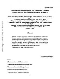
First, we examine the convergence behavior of inner iterations for updating x ¯ and C, i.e., (4.3) and (4.4), ¯ 0 and H 1 -prior C0 = 2.5 × 10⁻³ C ¯ 1 . To for the example phillips with the L2 -prior C0 = 1.0 × 10⁻¹ C 1 2 study the convergence, we fix C at C = I for x ¯ and present the ` -norm of the update δ¯ x (initialized with x ¯0 = 0), and similarly fix x ¯ at the converged iterate x ¯1 for C and present the spectral norm of the change δC. For both (4.3) and (4.4), these initial guesses are quite far away from the solutions, and thus the choice allows showing their global convergence behavior. The convergence is fairly rapid and steady for both inner iterations, cf. Fig. 1. For example, for a tolerance 10−5 , the Newton method (4.3) converges after about 10 iterations, and the fixed point method (4.4) converges after 4 iterations, respectively. The global as well as local superlinear convergence of the Newton method (4.3) are clearly observed, confirming the discussions in Section 4. The convergence behavior of the inner iterations is similar for both priors. In practice, it is unnecessary to solve the inner iterates to a very high accuracy, and it suffices to apply a few inner updates within each outer iteration. Since the iteration (4.4) often converges faster than (4.1), we take five Newton updates and one fixed point update per outer iteration for the numerical experiments below.
100
100
kδ¯ xk kδCk
10-6
10-6
10-12
10-12
10-18
1
5
10
10-18
15
kδ¯ xk kδCk
1
5
k
10
15
k
(a) L2 -prior
(b) H 1 -prior
Figure 1: The convergence of the inner iterations of Algorithm 1 for phillips.
kδ¯ xk kδCk
100
10-5
10-10
kδ¯ xk kδCk
100
10-5
1
2
3 k
4
10-10
5
(a) L2 prior
1
2
3 k
4
5
(b) H 1 -prior
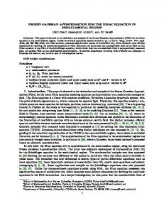
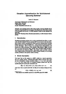
Figure 2: The convergence of outer iterations of Algorithm 1 for phillips. To examine the convergence of outer iterations, we show the errors of the mean x ¯ and covariance C and the lower bound F (¯ x, C) in Figs. 2 and 3, respectively. Algorithm 1 is terminated when the change of the lower bound falls below 10−10 . For the L2 -prior, Algorithm 1 converges after 5 iterations and the 15
3 0 ×10
×104
lower bound
lower bound
0
-1
-2
-4 -2 0
1
2
3
4
5
0
1
2
k
3
4
5
k
(a) L2 -prior
(b) H 1 -prior
Figure 3: The convergence of the lower bound F (¯ x, C) for phillips. last increments δ¯ x and δC are of order 10−8 and 10−9 , respectively. This observation holds also for the 1 H -prior, cf. Figs. 2(b) and 3(b). Thus, both inner and outer iterations converge rapidly and steadily, and Algorithm 1 is very efficient.
6.2
Low-rank approximation of A and sparsity of C
The discussions in Section 4.2 show that the structure on A and C can be leveraged to reduce the complexity of Algorithm 1. Now we evaluate their influence on the accuracy of the VGA. First, we examine the influence of low-rank approximation to A. Since the kernel function of the example phillips is smooth, the inverse problem is mildly ill-posed and the singular values σk decay algebraically, cf. Fig. 4(a). A low-rank matrix Ar of rank r ≈ 10 can already approximate A well. To study its influence on the VGA, we denote by (¯ xr , Cr ) and (¯ x∗ , C∗ ) the VGA for Ar and A, respectively. ∗ ∗ The errors ex¯ = k¯ xr − x ¯ k and eC = kCr − C k for different ranks r are shown in Figs. 4 (b) and (c) for the L2 - and H 1 -prior, respectively. Too small a rank r of the approximation Ar can lead to pronounced errors in both the mean x ¯ and the covariance C, whereas for a rank of r = 10, the errors already fall below one percent. Interestingly, the decay of the error ex¯ is much faster than that of the singular values σk , and the error eC decays slower than ex¯ . The fast decay of the errors ex¯ and eC indicates the robustness of the VGA, which justifies using low-rank approximations in Algorithm 1. 102 0
10-5
-2
10-5
10-10
10-4 10-6
ex¯ eC
error
10
100 ex¯ eC
error
σk
10
100
0
25
50 k
75
(a) singular values σk
100
10-15
10-10
0
25
50 r
(b) L2 -prior
75
100
10-15
0
25
50 r
75
100
(c) H 1 -prior
Figure 4: (a) singular values and (b)–(c): the errors of the mean and covariance for phillips. Next we examine the influence of the sparsity assumption on the covariance C, which is used to reduce the complexity of Algorithm 1. Due to the coupling between x ¯ and C, cf. (4.1)–(4.2), the sparsity assumption on C affects the accuracy of both x ¯ and C. To illustrate this, we take different sparsity
16
levels s on C in Algorithm 1, i.e., at most s nonzero entries around the diagonal of C. Surprisingly, a diagonal C already gives an acceptable approximation measured by the errors ex¯ = k¯ xs − x ¯∗ k2 and ∗ eC = kCs − C k2 , where (¯ xs , Cs ) is the VGA with a sparsity level s. The errors ex¯ and eC decrease with the sparsity level s, cf. Table 1. Thus the sparsity assumption on C can reduce significantly the complexity while retaining the accuracy. Table 1: The errors ex¯ and eC v.s. the sparsity level s of C for phillips. L2 prior ex¯ eC
prior s 1 3 5
6.3
6.38e-2 5.62e-2 4.88e-2
H 1 prior ex¯ eC
9.20e-2 8.10e-2 7.02e-2
1.92e-2 1.27e-2 1.00e-2
7.06e-2 5.42e-2 4.29e-2
Hierarchical parameter choice
Now we examine the convergence of Algorithm 2 for choosing the parameter α in the prior p(x). By Theorem 5.1, the sequence {αk } generated by Algorithm 2 is monotone. We illustrate this by two initial guesses, i.e., α1 = 0.1 and α1 = 10. Both sequences of iterates generated by Algorithm 2 converge monotonically to the limit α∗ = 0.7778, and the convergence of Algorithm 2 is fairly steady, cf. Fig. 5(a). Further, Algorithm 2 indeed maximizes the joint lower bound (5.1) with its maximum attained at α∗ = 0.7778, cf. Fig. 5(b). Though not shown, the lower bound Fα (¯ x, c|α) is also increasing during the iteration. Thus, the hierarchical approach is indeed performing model selection by maximizing ELBO. -200 joint lower bound
α
10
1 α*
-220 -240 -260
0.1 50
100
10-1
150
k
(a) convergence of α
100 α
101
(b) joint lower bound
Figure 5: (a)The convergence of Algorithm 2 initialized with 0.1 and 10, both convergent to α∗ = 0.7778 (b) the joint lower bound versus α, for phillips with L2 -prior. To illustrate the quality of the automatically chosen parameter α, we take six realizations of the Poisson data y and compare the mean x ¯ of the VGA with the optimal regularized solutions, where α is tuned so that the error is smallest (and thus it is infeasible in practice). The means x ¯ by Algorithm 2 are comparable with the optimal ones, cf. Fig. 6, and thus the hierarchical approach can yield reasonable approximations. The parameter α by the hierarchical approach is slightly smaller than the optimal one, cf. Table 2, and hence the corresponding reconstruction tends to be slightly more oscillatory than the optimal one. The value of the parameter α by the hierarchical approach is relatively independent of the realization, whose precise mechanism is to be ascertained.
17
0.8
0.8 exact opt Alg 2
0.4 x
x
0.4
0.6
0.2
0.2
0.4 0.2
0
0
0
-0.2
-0.2
-0.2
0
50 i
100
0
0.8
100
0
0.8 exact opt Alg 2
0.6 0.4 x
0.4 0.2
0.4
0.2
0.2
0
0
0
-0.2
-0.2
50 i
100
100
0
50 i
100
exact opt Alg 2
0.6
-0.2 0
50 i
0.8 exact opt Alg 2
x
0.6
x
50 i
exact opt Alg 2
0.6
x
0.6
0.8 exact opt Alg 2
0
50 i
100
Figure 6: The mean x ¯ of the Gaussian approximation by Algorithm 2 (Alg2) and the “optimal” solution (opt) for 6 realizations of Poisson data for phillips with the L2 -prior. Table 2: The values of the hyperparameter α for the results in Fig. 6. case opt Alg 2
6.4
1 2.64 0.78
2 3.35 0.76
3 2.59 0.76
4 1.35 0.77
5 9.31 0.73
6 4.04 0.74
VGA versus MCMC
Despite the widespread use of variational type techniques in practice, the accuracy of the approximations is rarely theoretically studied. This has long been a challenging issue for approximate Bayesian inference, including the VGA. In this part, we conduct an experiment to numerically validate the VGA against the results by Markov chain Monte Carlo (MCMC). To this end, we employ the standard MetropolisHastings algorithm, with the Gaussian approximation from the VGA as the proposal distribution (i.e., independence sampler). In other words, we correct the samples drawn from VGA by a Metropolis-Hastings step. The length of the MCMC chain is 2 × 10⁵ , and the last 1 × 10⁵ samples are used for computing the summarizing statistics. The acceptance rate in the Metropolis-Hastings algorithm is 96.06%. This might be attributed to the fact that the VGA approximates the posterior distribution fairly accurately, and thus nearly all the proposals are accepted. The numerical results are presented in Fig. 7, where the mean and the 90% highest posterior density (HPD) credible set are shown. It is observed that the mean and HPD regions by MCMC and VGA are very close to each other, cf. Figs. 7 and 8, thereby validating the accuracy of the VGA. The `2 error between the mean by MCMC and GVA is 9.80 × 10⁻³ , and the error between corresponding covariance in spectral norm is 6.40 × 10⁻³ . Just as expected, graphically the means and covariances are indistinguishable, cf. Fig. 8.
6.5
Numerical reconstructions
Last, we present VGAs for one- and two-dimensional examples. The numerical results for the following four 1D examples, i.e., phillips, foxgood, gravity and heat, for both L2 - and H 1 -priors, are presented in Figs. 9-12. For the example phillips with either prior, the mean x ¯ by Algorithm 1 agrees very
18
(a) MCMC
(b) VGA
¯ 0. Figure 7: The mean and 90% HPD by (a) MCMC and (b) VGA for phillips with C0 = 1.00 × 10⁻¹ C 0.8 exact posterior vga
0.6
x
0.4 0.2 0 -0.2 0
20
40
60
80
0.09
0.09
0.08
0.08
0.07
0.07
0.06
0.06
0.05
0.05
0.04
0.04
0.03
0.03
0.02
0.02
0.01
0.01
0
0
100
i
(a) mean
(b) MCMC
(c) VGA
Figure 8: (a) The mean by MCMC and VGA versus the exact solution, and the covariance by (b) MCMC ¯ 0. and (c) VGA for phillips with C0 = 1.00 × 10⁻¹ C well with the true solution x† . However, near the boundary, the mean x ¯ is less accurate. This might be attributed to the fact that in these regions, the Poisson count is relatively small, and it may be insufficient for an accurate recovery. For the L2 -prior, the optimal C is diagonal dominant, and decays rapidly away from the diagonal, cf. Fig. 9(b). For the H 1 -prior, C remains largely diagonally dominant, but the off-diagonal entries decay a bit slower. Thus, it is valid to assume that C is dominated by local interactions as in Section 4.2. These observations remain largely valid for the other 1D examples, despite that they are much more ill-posed. ×10 -3
0.8
0.8 exact mean
0.6
0.08
0.6
0.04
0
0.02
-0.2 25
50 i
75
0.4 5
0.2
0
0
0
100
15
10
x
0.06
0.2
x
0.4
0
exact mean
0
¯0 (a) C0 = 1.00 × 10⁻¹ C
25
50 i
75
100
¯1 (b) C0 = 2.5 × 10⁻³ C
Figure 9: The Gaussian approximation for phillips. Last, we test Algorithm 1 on a 2D image of size 128×128. In this example, the matrix A ∈ R16384×16384 is a (discrete) Gaussian blurring kernel with a blurring width 99, variance 1.5 and a circular boundary 19
1.5
1 exact mean
exact mean
10
0.8
0.2 0.15
8
1
0.6 0.1
x
x
6
0.4
0.5
0.05
4
0.2
0
2
0
0 0
25
50 i
75
0
100
-0.05
0
25
¯0 (a) C0 = 1.12 × 101 C
50 i
75
100
¯1 (b) C0 = 9.8 × 10⁻³ C
Figure 10: The Gaussian approximation for foxgood. 0.8
×10 -3
0.8 exact mean
0.6
0.08
exact mean
0.6 x
x
0.4
0.4
6
0.04
4
0.2
0.2
2
0.02
0
25
50 i
75
0
0
0
100
10 8
0.06
0
12
0
25
¯0 (a) C0 = 1 × 10⁻¹ C
50 i
75
100
-2
¯1 (b) C0 = 1.5 × 10⁻³ C
Figure 11: The Gaussian approximation for gravity. 6
6 exact mean
4
exact mean
0.8
4
1 0.8
x
x
0.6
2
0.4
0.6
2
0.4
0
0
0.2
0.2 0
-2 0
25
50 i
75
-2
100
0
¯0 (a) C0 = 3.2 × 10⁻¹ C
25
50 i
75
100
0
¯1 (b) C0 = 1 × 100 C
Figure 12: The Gaussian approximation for heat. condition. Since the blurring width is large, the matrix A is indeed low-rank, and we employ a rSVD approximation of rank 2000, where the rank is determined by inspecting the singular value spectrum. The true solution x† consists of two Gaussian blobs, cf. Fig. 13(a), and thus we employ a smooth prior with C0 = 6.00 × 10⁻² L−1 L−t , where L = I ⊗ L1 + L1 ⊗ I is the 2D first-order finite difference matrix. Since the problem size is very large, we restrict C to be a sparse matrix such that every pixel interacts only with at most four neighboring pixels. This allows reducing the computational cost greatly. The mean x ¯ is nearly identical with the true solution x† , and the error is very small, cf. Fig. 13. The structural similarity index between the mean x ¯ and the exact solution x† is 0.812. We also compare the VGA solution with the MAP estimator. The `2 error of the mean of the VGA is 9.7205, which is slightly smaller than that of the MAP estimator (9.7355). To indicate the uncertainty around the mean x ¯, we show in Fig. 13(f) the diagonal entries of C (i.e., the variance at each pixel). The variances are relatively large at pixels where the mean x ¯ is less accurate. In summary, the VGA can provide a reliable point estimator together with useful covariance estimates.
7
Conclusions
In this work, we have presented a study of the variational Gaussian approximation to the Poisson data (under the log linear link function) with respect to the Kullback-Leibler divergence. We derived explicit
20
3
35
3
2
25
2
1
15
1
128
0 -0.5 128
96
64
32
0
128
5 0 128
64 0
(a) true solution x†
96
64
32
0
128
0 -0.5 128
64 0
64 96
(b) Poisson sample y
3
2
2
1
1
32
0
0
(c) MAP xMAP 10
3
64
-3
12 10 8
128
0 -0.5 128
64 96
64
32
0
0
(d) mean x ¯
6 128
0 -0.5 128
64 96
64
32
0
0
(e) error x† − x ¯
4 2 128
128 64 96
64
32
0
0
(f) variance diag(C)
Figure 13: The Gaussian approximation for image deblurring. expressions for the lower bound functional and its gradient, and proved its strict concavity and existence and uniqueness of an optimal Gaussian approximation. Then we developed an efficient algorithm for maximizing the functional, discussed its convergence properties, and described practical strategies for reducing the complexity per iteration. Further, we analyzed hierarchical modeling for automatically determining the hyperparameter using the variational Gaussian approximation, and proposed a monotonically convergent algorithm for the joint estimation. These discussions were supported by extensive numerical experiments. There are several avenues for further study. First, one of fundamental issues is the quality of the Gaussian approximation relative to the true posterior distribution. In general this issue has been long standing, and it also remains to be analyzed for the Poisson model. Second, the variational Gaussian approximation can be viewed as a nonstandard regularization scheme, by also penalizing the covariance. This naturally motivates the study on its regularizing property from the perspective of classical regularization theory, e.g., consistency and convergence rates. Third, the approach generally gives a very reasonable approximation. This suggests itself as a preconditioner for sampling techniques, e.g., variational approximation as the proposal distribution (i.e., independence sampler) in the standard Metropolis-Hastings type algorithm or as the base distribution for importance sampler. It is expected to significantly speed up the convergence of these sampling procedures, which is confirmed by the preliminary experiments. We plan to study these aspects in future works.
Acknowledgements The work of B. Jin is supported by UK EPSRC grant EP/M025160/1, and that of C. Zhang by a departmental studentship.
21
A
On the iteration (4.4)
In this appendix, we discuss an interesting property of the iteration (4.4), for the initial guess C0 = C0 . We denote the fixed point map in (4.4) by T, i.e., t
1
t A¯ x+ 2 diag(ACA ) T(C) = (C−1 )A)−1 . 0 + A diag(e + ˜ ∈ S + , if 0 ≤ C ≤ C, ˜ The next result gives the antimonotonicity of the map T on Sm , i.e., for C, C m ˜ then T(C) ≥ T(C).
Lemma A.1. The mapping T is antimonotone. ˜ ∈ S + . If C ≤ C, ˜ then diag(ACAt ) ≤ diag(ACA ˜ t ) componentwise. The claim follows Proof. Let C, C m t t 1 ˜ ) ˜ = T(C)At diag(eA¯x+ 12 diag(ACA ˜ ≥ 0. from the identity T(C) − T(C) − eA¯x+ 2 diag(ACA ) )AT(C) The next result shows the monotonicity of the sequence {Ck } generated by (4.4). + Lemma A.2. For any initial guess C0 ∈ Sm , the sequence {Ck }k≥0 generated by the iteration (4.4) has k the following properties: (i) C ≥ 0 for all k ≥ 0; (ii) Ck ≤ C0 for all k ≥ 0; (iii) If Ck ≥ Cj then Ck+1 ≤ Cj+1 ; (iv) If Ck ≥ Cj then Ck+2 ≥ Cj+2 .
Proof. Properties (i) and (ii) are obvious. Properties (iii) and (iv) are direct consequences of the fact + , cf. Lemma A.1. that the map T is antimonotone on Sm The next result shows that the sequence constitutes two subsequences, each converging to a fixed point of T2 , which implies either a periodic orbit of period 2 of the map T or a fixed point of T, Theorem A.1. With the initial guess C0 = C0 , the sequence {Ck }k≥0 generated by iteration (4.4) converges to a fixed-point of T2 . Proof. Lemma A.2(ii) implies C2 ≤ C0 ,
(A.1)
so we can use Lemma A.2(iv) inductively to argue that {C2k }k≥0 is a decreasing sequence. From (A.1) and Lemma A.2(iii), we deduce C1 ≤ C3 , which together with Lemma A.2(iv) implies that the sequence {C2k+1 }k≥0 is increasing. By the boundedness and monotonicity, both {C2k }k≥0 and {C2k+1 }k≥0 converge, with the limit C∗ and C∗∗ , respectively. These are the limits of the fixed point map T2 . Remark A.1. By Lemma A.2, C∗ ≥ C∗∗ , and if C∗ = C∗∗ , the whole sequence converges. Generally, the interval of matrices [C∗∗ , C∗ ] provides a lower and sharp bounds for the fixed point of the iteration (4.4) (which is a priori known to be unique and to exist). By repeating the argument in [10, Theorem 2.2], one may also examine the convergence of the sequence for the initial guess either C0 < C∗∗ or C0 > C∗ .
B
Differentiability of the regularized solution
In this part, we discuss the differentiability of the regularized solution (¯ xα , Cα ) in α. For simplicity, we d¯ x ˙ = dC ): ¯˙ = dα omit the subscript α. By differentiating (3.6) in α and chain rule, we obtain (with x and C dα ˙ t ) = −C ¯ −1 (¯ ¯˙ + 12 At Ddiag(ACA x − µ0 ), (At DA + αC−1 0 )x 0 1
1
1
1
˙ −1 + 1 At D 2 diagdiag(ACA ˙ t )D 2 A) + At D 2 diag(Ax ¯ −1 , ¯˙ )D 2 A = −C (C−1 CC 0 2 1
t
(B.1)
where D = diag(eA¯x+ 2 diag(ACA ) ) ∈ Rn×n is a diagonal matrix. This constitutes a coupled linear system ˙ The next result gives its unique solvability. ¯˙ , C). for (x Theorem B.1. The sensitivity system (B.1) is uniquely solvable. 22
Proof. Since the system (B.1) is linear and square, it suffices to show that the homogeneous problem has ¯˙ from the second line in (B.1) using the only a zero solution. To this end, by eliminating the variable x ˙ first line, we obtain the Schur complement for C: 1
1
1
1
˙ t )D 2 A − 1 At D 2 diag(A(At DA + αC ¯ −1 )−1 At Ddiag(ACA ˙ −1 + 1 At D 2 diagdiag(ACA ˙ t ))D 2 A. C−1 CC 0 2 2 For any fixed C, this defines a linear map on Rm×m . Next we show its invertibility. To this end, we take ˙ and show its positivity. Clearly, the first term is strictly positive. Thus it inner product the map with C, suffices to consider the last two terms. By the cyclic property of trace, with d = diag(D) ∈ Rn , we have ˙ t ))A, C) ˙ = tr(At diag(d ◦ diag(ACA ˙ t ))AC) ˙ (At diag(d ◦ diag(ACA ˙ t )), ACA ˙ t ) = (Ddiag(ACA ˙ t ), diag(ACA ˙ t )) = (¯ ¯), =(Ddiag(diag(ACA e, e 1 ˙ t ) ∈ Rn . Similarly, by letting A ¯ = D 21 A, we have where ¯ e = D 2 diag(ACA
t ¯ −1 )−1 At Ddiag(ACA ˙ t ))A, C) ˙ (At Ddiag(A(A DA + αC 0 ¯ −1 )−1 At Ddiag(ACA ˙ t )), ACA ˙ t) =(Ddiag(A(At DA + αC 0
¯ A ¯ tA ¯ + αC ¯ −1 )−1 A ¯ te ¯, e ¯). =(A( 0 ¯ A ¯ tA ¯ + αC ¯ −1 )−1 A ¯ t > 0, the associated bilinear form is coercive on S + . Thus the Schur Since In − A( m 0 complement is invertible, and the system (B.1) has a unique solution. ˙ 6= 0. Corollary B.1. For any rank deficient A, C 1 ˙ = 0, the second equation in (B.1) reduces to At D 12 diag(Ax ¯ −1 . By assumption, ¯˙ )D 2 A = −C Proof. If C 0 A is rank deficient, and thus the left hand side is rank deficient, whereas the right hand side is of full ˙ 6= 0. rank, which leads to a contradiction. Thus we have C
The next result gives a lower-bound for the derivative
d xα , Cα ). dα ψ(¯
Theorem B.2. The functional ψ(¯ xα , Cα ) satisfies d ˙ −1 , C). ˙ ¯˙ , x ¯˙ ) + 12 (C−1 CC ψ(¯ xα , Cα ) ≥ α(C−1 0 x dα Proof. By the definition of the functional ψ, we have d ¯ −1 (¯ ¯ −1 , C). ˙ ¯˙ ) − 21 (C ψ(¯ xα , Cα ) = −(C x − µ0 ), x 0 0 dα ˙ we get ¯˙ , and the second with 21 C, By taking inner product the first equation in (B.1) with x ˙ t ), x ¯ −1 (¯ ¯˙ , x ¯˙ ) + 12 (At Ddiag(ACA ¯˙ ) = −(C ¯˙ ), ((At DA + αC−1 x − µ0 ), x 0 )x 0 −1 ˙ 1 CC−1 2 (C
1 1 ˙ t )D 21 A, C) ˙ + 1 (At D 12 diag(Ax ˙ = − 1 (C ¯ −1 , C). ˙ ¯˙ )D 2 A, C) + 12 At D 2 diagdiag(ACA 0 2 2
By the cyclic property of trace and summing these two identities, we obtain ¯ −1 (¯ ¯ −1 , C) ˙ =(αC−1 x ˙ −1 , C) ˙ ˙ ¯˙ ) + 12 (C−1 CC ¯˙ ) − 12 (C −(C x − µ0 ), x 0 0 0 ¯, x ˙ t ), diag(ACA ˙ t )) ¯˙ , x ¯˙ ) + 1 (Ddiag(ACA + (At DAx 4 t
1 2
1 2
˙ ), D Ax ¯˙ ). + (D diag(ACA Meanwhile, by the Cauchy-Schwarz inequality, we have 1
1
1
1
1
1
˙ t ), D 2 Ax ˙ t ), D 2 diag(ACA ˙ t )). ¯˙ ) ≥ −(D 2 Ax ¯˙ , D 2 Ax ¯˙ ) − 14 (D 2 diag(ACA (D 2 diag(ACA Substituting the preceding inequality into (B.2) yields the desired estimate. 23
(B.2)
Corollary B.2. The functional ψ(¯ xα , Cα ) is strictly increasing in α. Proof. By Theorem B.1, (B.1) is uniquely solvable. Since the right hand side of (B.1) is nonvanishing ˙ to (B.1) is nonzero. Thus, by Theorem B.2, ¯˙ , C) (by assumption, C0 is nonzero), the solution pair (x d xα , Cα ) is strictly positive, i.e., ψ(¯ xα , Cα ) is strictly increasing. dα ψ(¯ Remark B.1. For the standard regularized least-squares problem, the solution is distinct for different α, and it never vanishes (except the trivial case y = 0). The proof in Corollary B.2 indicates that an analogous statement holds for the Poisson model (2.2).
References [1] W. N. Anderson, Jr., G. B. Kleindorfer, P. R. Kleindorfer, and M. B. Woodroofe. Consistent estimates of the parameters of a linear system. Ann. Math. Stat., 40:2064–2075, 1969. [2] C. Archambeau, D. Cornford, M. Opper, and J. Shawe-Taylor. Gaussian process approximations of stochastic differential equations. JMLR: Workshop Conf. Proc., 1:1–16, 2007. [3] D. Barber and C. M. Bishop. Ensemble learning in Bayesian neural networks. NATO ASI Series F Comput. Syst. Sci., 168:215–238, 1998. [4] J. M. Bardsley and A. Luttman. A Metropolis-Hastings method for linear inverse problems with Poisson likelihood and Gaussian prior. Int. J. Uncertain. Quantif., 6(1):35–55, 2016. [5] D. P. Bertsekas. Nonlinear Programming. Athena Scientific, Belmont, MA, second edition, 1999. [6] C. M. Bishop. Pattern Recognition and Machine Learning. Springer, Singapore, 2006. [7] A. Cameron and P. K. Trivedi. Regression Analysis of Count Data. Cambridge University Press, 1998. [8] E. Challis and D. Barber. Gaussian Kullback-Leibler approximate inference. J. Mach. Learn. Res., 14(1):2239–2286, 2013. [9] P. S. Dwyer. Some applications of matrix derivatives in multivariate analysis. J. Amer. Stat. Assoc., 62(318):607–625, 1967. [10] S. M. El-Sayed and A. C. M. Ran. On an iteration method for solving a class of nonlinear matrix equations. SIAM J. Matrix Anal. Appl., 23(3):632–645, 2001/02. [11] H. W. Engl, M. Hanke, and A. Neubauer. Regularization of Inverse Problems. Kluwer Academic, Dordrecht, 1996. [12] H. Erdoˇ gan and J. A. Fessler. Monotonic algorithms for transmission tomography. IEEE Trans. Med. Imag., 18(9):801–814, 1999. [13] B. G¨ artner and J. Matousek. Approximation Algorithms and Semidefinite Programming. SpringerVerlag, Berlin, Heidelberg,, 2012. [14] G. H. Golub and C. F. Van Loan. Matrix Computations. Johns Hopkins University Press, Baltimore, MD, fourth edition, 2013. [15] N. Halko, P.-G. Martinsson, and J. A. Tropp. Finding structure with randomness: Probabilistic algorithms for constructing approximate matrix decompositions. SIAM Rev., 53(2):217–288, 2011. [16] P. Hall, J. T. Ormerod, and M. P. Wand. Theory of Gaussian variational approximation for a Poisson mixed model. Stat. Sinica, 21(1):369–389, 2011.
24
[17] G. E. Hinton and D. Van Camp. Keeping the neural networks simple by minimizing the description length of the weights. In COLT’93, Proc. 6th Annual Conf. Comput. Learning Theory, pages 5–13, New York, 1993. ACM. [18] T. Hohage and F. Werner. Inverse problems with Poisson data: statistical regularization theory, applications and algorithms. Inverse Problems, 32(9):093001, 56, 2016. [19] K. Ito and B. Jin. Inverse Problems: Tikhonov Theory and Algorithms. World Scientific, Hackensack, NJ, 2015. [20] K. Ito, B. Jin, and T. Takeuchi. A regularization parameter for nonsmooth Tikhonov regularization. SIAM J. Sci. Comput., 33(3):1415–1438, 2011. [21] W. James and C. Stein. Estimation with quadratic loss. In Proc. 4th Berkeley Sympos. Math. Statist. and Prob., Vol. I, pages 361–379. Univ. California Press, Berkeley, Calif., 1961. [22] B. Jin and J. Zou. Augmented Tikhonov regularization. Inverse Problems, 25(2):025001, 25, 2009. [23] J. Kaipio and E. Somersalo. Statistical and Computational Inverse Problems. Springer-Verlag, New York, 2005. [24] R. E. Kass and A. E. Raftery. Bayes factors. J. Amer. Stat. Assoc., 90(430):773–795, 1995. [25] C. T. Kelley. Iterative Methods for Linear and Nonlinear Equations. SIAM, Philadelphia, PA, 1995. [26] M. E. Khan, S. Mohamed, and K. Murphy. Fast Bayesian inference for nonconjugate Gaussian process regression. In NIPS, pages 3140–3148, 2012. [27] B. Kulis, M. A. Sustik, and I. S. Dhillon. Low-rank kernel learning with Bregman matrix divergences. J. Mach. Learn. Res., 10:341–376, 2009. [28] S. Kullback and R. A. Leibler. On information and sufficiency. Ann. Math. Stat., 22:79–86, 1951. [29] Y. Lu, A. M. Stuart, and H. Weber. Gaussian approximations for probability measures on Rd . SIAM/ASA J. Uncertainty Quantification, in press. arXiv:1611.08642, 2016. [30] T. P. Minka. Expectation propagation for approximate Bayesian inference. In Proc. 17th Conf. Uncertainty in Artificial Intelligence, pages 362–369. Morgan Kaufmann Publishers Inc., 2001. [31] M. Opper and C. Archambeau. The variational Gaussian approximation revisited. Neural Comput., 21(3):786–792, 2009. [32] J. T. Ormerod and M. P. Wand. Gaussian variational approximate inference for generalized linear mixed models. J. Comput. Graph. Statist., 21(1):2–17, 2012. [33] J. Pillow. Likelihood-based approaches to modeling the neural code. In K. Doya, S. Ishii, A. Pouget, and R. Rao, editors, Bayesian Brain: Probabilistic Approaches to Neural Coding, pages 53–70. MIT Press, Cambridge, 2007. [34] F. J. Pinski, G. Simpson, A. M. Stuart, and H. Weber. Kullback-Leibler approximation for probability measures on infinite-dimensional spaces. SIAM J. Math. Anal., 47(6):4091–4122, 2015. [35] P. Ravikumar, M. J. Wainwright, G. Raskutti, and B. Yu. High-dimensional covariance estimation by minimizing `1 -penalized log-determinant divergence. Electron. J. Stat., 5:935–980, 2011. [36] D. Rohde and M. P. Wand. Semiparametric mean field variational Bayes: general principles and numerical issues. J. Mach. Learn. Res., 17:Paper No. 172, 47, 2016.
25
[37] T. Schuster, B. Kaltenbacher, B. Hofmann, and K. S. Kazimierski. Regularization Methods in Banach Spaces. Walter de Gruyter GmbH & Co. KG, Berlin, 2012. [38] A. M. Stuart. Inverse problems: a Bayesian perspective. Acta Numer., 19:451–559, 2010. [39] L. Tierney and J. B. Kadane. Accurate approximations for posterior moments and marginal densities. J. Amer. Stat. Assoc., 81(393):82–86, 1986. [40] M. J. Wainwright and M. I. Jordan. Graphical models, exponential families, and variational inference. c Found. Trends Mach. Learn., 1(1–2):1–305, 2008. [41] M. Yavuz and J. A. Fessler. New statistical models for randoms-precorrected PET scans. In Information Processing in Medical Imaging (Lecture Notes in Computer Science), volume 1230, pages 190–203. Springer-Verlag, 1997. [42] Y. Zhang and W. E. Leithead. Approximate implementation of the logarithm of the matrix determinant in Gaussian process regression. J. Stat. Comput. Simul., 77(4):329–348, 2007.
26