QUT Digital Repository: http://eprints.qut.edu.au/
McGrory, Clare A. and Titterington, D. M. and Reeves, Robert W. and Pettitt, Anthony N. (2008) Variational Bayes for estimating the parameters of a hidden Potts model. Statistics and Computing In Press.
© Copyright 2008 Springer The original publication is available at SpringerLink http://www.springerlink.com
Variational Bayes for Estimating the Parameters of a Hidden Potts Model C.A. McGrory, D.M. Titterington, R. Reeves, A.N. Pettitt Abstract Hidden Markov random field models provide an appealing representation of images and other spatial problems. The drawback is that inference is not straightforward for these models as the normalisation constant for the likelihood is generally intractable except for very small observation sets. Variational methods are an emerging tool for Bayesian inference and they have already been successfully applied in other contexts. Focusing on the particular case of a hidden Potts model with Gaussian noise, we show how variational Bayesian methods can be applied to hidden Markov random field inference. To tackle the obstacle of the intractable normalising constant for the likelihood, we explore alternative estimation approaches for incorporation into the variational Bayes algorithm. We consider a pseudo-likelihood approach as well as the more recent reduced dependence approximation of the normalisation constant. To illustrate the effectiveness of these approaches we present empirical results from the analysis of simulated datasets. We also analyse a real dataset and compare results with those of previous analyses as well as those obtained from the recently developed auxiliary variable MCMC method and the recursive MCMC method. Our results show that the variational Bayesian analyses can be carried out much faster than the MCMC analyses and produce good estimates of model parameters. We also found that the reduced dependence approximation of the normalisation constant outperformed the pseudo-likelihood approximation in our analysis of real and synthetic datasets. Keywords: Potts/Ising model, Hidden Markov random field, variational approximation, Bayesian inference, pseudo-likelihood, reduced dependence approximation 1
Affiliation of Authors
C.A.McGrory Corresponding author: School of Mathematical Sciences, Queensland University of Technology, GPO Box 2434, Brisbane, Queensland, 4001, Australia, Tel. (61)7-3138-1287, Fax.: (61)7-3138-2310,
[email protected]. D.M. Titterington University of Glasgow R. Reeves Queensland University of Technology A.N. Pettitt Queensland University of Technology
2
1
Introduction
Markov random fields (MRFs) are spatial models whose spatial locations or sites generally follow some sort of lattice structure. In a discrete Markov random field, the observation at each of these sites belongs to one of K, say, possible states. Each site on the lattice has a set of neighbouring sites and the attractiveness of such models lies in the fact that the conditional probability at each site is dependent only upon the values of its neighbours. This structure is useful in a variety of research areas where there is an interest in representing the spatial association between data. Some examples are medical imaging, environmental statistics and genetics. Usually in practical applications it is not clear to which state a given observation belongs, and in some cases even the number of states is unknown. In this setting, the hidden Markov random field (HMRF) representation is an appropriate one. HMRFs have been used in various areas where interest lies in modelling spatial dependency between regions or objects which are geographically close to one another or which are related in some other way. Image analysis is an important application area for HMRFs, the work by Geman and Geman (1984) and Besag (1986) having been influential in this. Recent application areas include micro-array data analysis (Gottardo et al. 2006), brain imaging (Smith and Fahrmeir 2006), disease mapping (Green and Richardson 2002) and agricultural field experiments (Besag and Higdon 1999). The Ising model for representing binary lattice data and its generalisation to categorical data, the Potts model, are two well-known and widely applied examples of a MRF-type model. These models originated in statistical physics but have been useful in many other modelling areas. This paper focuses on Bayesian inference in the case where the hidden data are represented by the Ising/Potts HMRF model. A difficulty with HMRF models, and hence the hidden Ising and Potts models, is that the normalising constant associated with the likelihood is generally intractable. This of course presents a problem in Bayesian inference as the computation of the likelihood is integral to the approach. A very recent development for Markov chain Monte Carlo (MCMC) algorithms for analysing distributions such as HMRFs with intractable normalising constants is presented in Møller et al. (2006). Møller et al. (2006) avoid the problem of estimating the normalising constant altogether by developing an auxiliary variable MCMC scheme in which the troublesome constant is cancelled out. This work is developed further by Murray et al. 3
(2006). This method produces accurate results but the drawback is that the computing time involved can be considerable. Many modern applications involve large data sets. Therefore, methods of analysis that are computationally efficient as well as accurate are very valuable. Approximate methods can often provide a time efficient solution to inference problems with only a small reduction in accuracy. In this paper we show how variational approximations, or variational Bayes, can be used to carry out Bayesian inference for estimating the parameters of a hidden Ising/Potts model. We use the auxiliary variable MCMC approach as a reference method with which we compare our results. Variational methods are non-simulation based and computationally efficient and their usefulness has already been demonstrated in other scenarios such as mixture model analysis (McGrory and Titterington 2006a, Corduneanu and Bishop 2001, Attias 1999) and hidden Markov chain analysis (McGrory and Titterington 2006b, MacKay 1997). Calculation of the posterior distribution of model parameters given observed data is a key objective in Bayesian analysis. This is not always straightforward as in many situations posterior distributions are intractable as is the case with HMRF models. The variational Bayes method provides a way of approximating such posteriors through the introduction of a simpler approximating function that is chosen to minimise the Kullback-Leibler divergence between the true and approximating function. However, as we have already mentioned, a difficulty which arises in the analysis of the hidden Potts model and other HMRF models, and hence in the variational Bayes scheme, is that the normalisation constant associated with the likelihood is usually intractable. This presents an obstacle for inference and consequently the investigation of normalising constant estimation techniques is an area of active research. Approaches include approximate methods such as thermodynamic integration, or path sampling (Gelman and Meng 1998, Pettitt et al. 2003). Reeves and Pettitt (2004) present an exact recursive method which enables calculation of the normalising constant for small lattices and this is extended in Friel et al. (2006) for application to larger lattices through an approximate method called the Reduced Dependence Approximation or RDA. In our variational Bayes scheme we employ the RDA method of Friel et al. (2006) to estimate the normalising constant and compare results with those obtained by taking a pseudo-likelihood approach (Besag 1974,1975,1986) at the relevant point in the variational
4
algorithm. Although the pseudo-likelihood may be a crude approximation, it is simplistic and can be computed quickly. For this reason we considered it an option worth exploring. In our analysis of the soil phosphate dataset, discussed in Section 5.2, we also compare our results with those obtained using the auxiliary variable MCMC approach of Møller et al. (2006) and the recursive method of Reeves and Pettitt (2004). In Section 2 we outline the fundamental principles of the variational Bayes approach. In Section 3 we describe the Ising and Potts models and discuss some methods for approximating the intractable normalising constant of the associated likelihood. In Section 4 we show how variational Bayes can be used to infer the parameters of a hidden Potts model in conjunction with the normalising constant approximations. Results of our analyses of synthetic and real data are presented in Section 5 with conclusions given in Section 6.
2
The Variational Bayes Approach
Suppose we have a missing data model with parameters θ and latent variables z. Calculation of the posterior distribution of the parameters θ, given the observed data y, is central to carrying out a Bayesian analysis. However, in many practical situations, posterior distributions cannot be computed exactly. In these situations, the variational Bayes method provides a means of approximating the intractable posterior. This is done by introducing a variational function q(θ, z) as an approximation to the joint posterior p(θ, z|y) from which the required posterior over the parameters can be found. To find an approximating function that is as close as possible to the true posterior, q(θ, z) is chosen to be the minimiser of the KullbackLeibler (KL) divergence between q(θ, z) and the joint posterior p(θ, z|y). The idea behind this is that minimising this KL divergence is the same as finding a rigorous lower bound on the log marginal likelihood. To see this, note that, by Jensen’s inequality, the log-likelihood can be lower bounded in the following way.
5
log p(y) = log
Z X
p(y, z, θ)dθ
{z}
= log ≥
Z X
Z X
q(θ, z)
{z}
q(θ, z) log
{z}
p(y, z, θ) dθ q(θ, z) p(y, z, θ) dθ. q(θ, z)
(1)
Since the difference between the two sides of the inequality (1) is given by the KL divergence, KL(q|p) =
Z X
q(θ, z) log
{z}
q(θ, z) dθ, p(θ, z|y)
it is evident that maximising the lower bound, (1), is equivalent to minimising the KL divergence between the two quantities. It is well known that the KL divergence is minimised by taking q(θ, z) = p(θ, z|y), but, in order to make any progress towards a solution, q(θ, z) must be computable. Therefore, to simplify matters we assume that q(θ, z) factorises over the parameters and latent values, leading to the distributional form q(θ, z) = qθ (θ)qz (z). The variational Bayes algorithm then proceeds to iteratively maximise (1) with respect to qθ (θ) and qz (z). At each iteration the lower bound is increased provided it is not already at a maximum. As a result of this similarity with the expectation maximisation (EM) algorithm, the algorithm is sometimes referred to as the variational Bayes expectation maximisation (VBEM) algorithm. Another outcome is that, when variational Bayes is applied to exponential-family models with the appropriate conjugate priors selected, the variational posterior for the model parameters will also belong to that conjugate family (for more detail on this point see, for example, Beal and Ghahramani (2003) or McGrory (2005)).
3
Hidden Markov Random Field Modelling
Consider a grid or lattice with regularly spaced sites i = 1, ..., n; in the context of image analysis, these sites correspond to pixels. Each site belongs to one of K states. For example, 6
these states might correspond to pixel colour when the lattice represents an image or, in a remote sensing problem, the states might correspond to land-use types. The true states z = {z1 , . . . , zn } are hidden and what we observe are noisy observations y = {y1 , . . . , yn }. The conditional probability at a given site depends only upon the values of neighbouring sites. In a first-order neighbourhood, the neighbours of a site are the sites above, below, to the left and to the right. The notation δi denotes the sites that are the neighbours of site i. We also use the notation i ∼ j to indicate that i and j are neighbours of one another. It is possible to consider higher-order neighbourhood systems but we do not do so in this paper. Increasing the order of the neighbourhood considered increases the amount of information used to estimate the true value of each pixel. This could improve the performance of inference techniques in some cases but would also increase computation time. The Hammersley-Clifford Theorem identifies MRFs with Gibbs distributions (see Besag 1974,1975, for example). This is a valuable result because it provides a straightforward way of specifying the distribution of a MRF. For this reason MRFs are usually defined through their representations as Gibbs distributions. Two well-studied examples of Gibbsian models that are often used to represent images are the Ising model and its generalisation, the Potts model.
3.1
The Ising Model and the Potts Model
The idea of the Ising model translates in a natural way to the binary image setting, representing the two colours present by +/-1 and assuming that nearby pixels are likely to have similar colour values. Suppose that the parameter of the MRF is β and that the variables zi , which represent the state or colour at a given pixel, take values in {−1, +1}. The Ising model is of the form P exp{β i∼j zi zj } p(z|β) = , G(β) where G(β) is a normalising constant which is usually not computable. The parameter β measures the strength of association between neighbouring pixels. Large positive values of β encourage neighbouring pixels to be of the same colour so that increasing β leads to bigger 7
patches of like-coloured pixels in the image. In 2 dimensions the Ising model undergoes a continuous phase transition at the critical value βc ≈ 0.44 and moves from a disordered to an ordered phase. The development of ordering occurs gradually as β increases above the critical value and, in our context, this means that when β is sufficiently above the critical value, the entire image will be made up of only one colour. For this reason, values of β that are too large would not be of interest here. This transition phenomenon is very important in statistical physics where the Ising model has its origins as a model for magnetic materials. For further detail see, for example, Newman and Barkema (1999). The natural extension of the Ising model to more than two states is given by the Potts model. In the Potts model each site can take more than two discrete values. For instance, a K-state Potts model is one in which each site can take values in states 1, . . . , K. The variables z corresponding to the states are K-vectors, zi = (zi1 , ..., ziK ), the elements of which take values in {0, 1} such that zil = 1 if and only if the observation at site i belongs to state l. Then p(z|β) =
exp{β
P
δ(zi , zj )} , G(β) i∼j
(2)
and
T
δ(zi , zj ) = 1, if zi zj =
K X
zil zjl = 1
l=1 T
= −1, otherwise, i.e. if zi zj =
K X
zil zjl = 0.
l=1
We can write δ(zi , zj ) = 2
K X
zil zjl − 1.
l=1
For K = 2 states, the Potts model is equivalent to the Ising model up to an additive constant.
8
3.2
The Hidden Potts Model
This paper focuses on the case where our data are modelled by a K-state hidden Potts Model with independent Gaussian noise. The joint probability distribution of y, z and θ is p(y, z, θ) = {
n Y
p(yi |zi , φ)}p(z|β){
i=1
K Y
p(φl )}p(β),
l=1
where θ = (φ, β). Here φ = (φ1 , . . . , φK ) where the φl ’s are parameters within the lth noise model and p(y, z, θ) =
" n K YY
# {p(yi |φl )}
i=1 l=1
zil
p(z|β){
K Y
p(φl )}p(β).
(3)
l=1
We assume that the lth noise model is N (µl , τl−1 ), with mean µl and where τl is the precision (τl−1 = σl2 ) so that φl = (µl , τl ).
3.3
Approximating the Normalising Constant
The normalising constant, also referred to as the partition function, for the likelihood of a HMRF cannot be evaluated exactly unless the observation set is very small. In this paper we consider two approaches to dealing with the issue of approximating the normalising constant of the hidden Potts/Ising model within the variational framework. The first of these is the reduced dependence approximation (RDA) to the normalising constant and the second is the pseudo-likelihood approach. The Reduced Dependence Approximation The RDA (Friel et al. 2006) extends the recursion method for normalising constant calculation, presented in Reeves and Pettitt (2004), to problems involving larger lattices. This results in an approximation to the true normalising constant. The recursive method (Reeves and Pettitt 2004) enables exact computation of the normalising constant for an unnormalised joint likelihood that can be expressed as a product of factors. As factorisation of the joint likelihood is applicable to any discrete Markov random field, the recursion method 9
is suitable for these models. However, it is only feasible when the lattice size is not too large, that is up to approximately 20 rows, with computing time increasing proportionally with the number of columns. The recursion method can be used to compute the normalising constant for the unnormalised likelihood, ϕ(z|β), of a HMRF as follows. Here ϕ(z|β) can be expressed in a factorised form as ϕ(z|β) = ϕ1 (z1 , z2 , ..., zr+1 |β)ϕ2 (z2 , z3 , ..., zr+2 |β) . . . ϕs (zs , zs+1 , ..., zn |β), where r < n and s = n − r. This is referred to as a lag-r model. Here r determines the degree of complexity or dependence of the model after optimal indexing of the z’s so as to make r as small as possible. Note that the exact grouping of the terms of the HMRF in the factorisation is not unique nor is it of consequence. For an example of a possible factorisation for a HMRF model see Reeves and Pettitt (2004). As a result of the above factorisation, the P normalising constant, G(β) = {z1 ,...,zn } ϕ(z|β), can be expressed as
G(β) =
X X zs+1 ...zn zs
ϕs (zs , zs+1 , ..., zn |β)
X
ϕs−1 (zs−1 , zs , ..., zn−1 |β) · · ·
zs−1
X
ϕ1 (z1 , z2 , ..., zr+1 |β).
z1
This expression can then be evaluated through forward recursion with a computation time significantly less than that of a straightforward summation over all possible realisations of the (z1 , . . . , zn ). Note that, when r = 1, the recursion method corresponds to the well-known forward-backward algorithm for hidden Markov models and so the recursion method is a generalisation of this result to a lattice. See Reeves and Pettitt (2004) for further detail on the recursive method. See also Jordan (2004) for an alternative perspective on this approach. The RDA provides a means of extending this approach to larger lattice sizes. It finds a close approximation to the true normalising constant through the relaxation of certain dependencies within the model. This involves approximating p(z|β) so that it can be expressed as a product of factors that are defined on sublattices. The normalising constants of these sublattices can be then computed using the recursive method described above allowing us to obtain an approximation to the true normalising constant as follows. We denote the vector 10
of states in row ρ by rρ and we denote by u0 , say, a number of rows which is smaller than the actual number of rows, u in the lattice. Then, making use of the Markov property and an approximation, we can approximate p(z|β) as
p(z|β) = p(ru−u0 +1 , ..., ru |β)
0 u−u Y
p(rρ |rρ+1 , β)
ρ=1
= p(ru−u0 +1 , ..., ru |β)
0 u−u Y
ρ=1
≈ p(ru−u0 +1 , ..., ru |β)
0 u−u Y
ρ=1
p(r1 , . . . , rρ |rρ+1 , β) p(r1 , . . . , rρ−1 |rρ , β) p(rp−u0 , . . . , rρ |β) . p(rp−u0 , . . . , rρ−1 |β)
(4)
The marginal probabilities in (4) can be approximated as p(rp−u0 , . . . , rρ |β) ≈
ϕ(rp−u0 , . . . , rρ |β) . G(u0 +1)×v (β)
In the above, v is the number of columns in the lattice, ϕ(rρ−u0 , . . . , rρ |β) represents the unnormalised distribution of the sub-lattice of dimension (u0 +1)×v defined on rows ρ−u0 , . . . , ρ of the lattice and G(u0 +1)×v (β) is the corresponding normalising constant of the sub-lattice. The above expression is an approximation because it ignores some of the associations between rows within the lattice. See Friel et al. (2006) for more detail on this point. Expressing each of the marginal distributions in (4) similarly leads to the approximation for the normalising constant 0
u−u ] = (G(u0 +1)×v (β)) 0 . G(β) ((Gu0 ×v (β))u−u −1
The normalising constants of these sub-lattices can be computed exactly via the recursive method when u0 is chosen to be reasonably small. The Pseudo-likelihood Approach This approach involves replacing the intractable likelihood, at appropriate stages, by the 11
pseudo-likelihood in the spirit of Ryd´en and Titterington (1998). The pseudo-likelihood is given by
pP L (z|β) = =
n Y i=1 n Y
p(zi |z−i , β) where z−i = {zj : j 6= i}, p(zi |zδi , β),
i=1
where zδi denotes the z-values of the pixels which are neighbours of pixel i. The normalising constants for the factors of the pseudo-likelihood are computable and so the unobtainable quantity has been replaced by something more amenable.
4
Variational Bayesian Analysis of a Hidden K-State Potts Model
We consider a K-state hidden Potts model with independent Gaussian noise and joint probability distribution given by (3) as described in Section 3.2. Assigning the Prior Distributions We assign independent Gaussian priors to the means µ = (µ1 , . . . , µK ), conditional on the precisions τ = (τ1 , . . . , τK ), so that p(µ|τ ) =
K Y
(0)
N (µl ; ml (0) , (λl τl )−1 ).
l=1
The precisions are given independent Gamma prior distributions: p(τ ) =
K Y
1 (0) 1 (0) Ga(τl ; γl , ξl ). 2 2 l=1 12
(0)
(0)
(0)
In the above, the {ml (0) }, {λl }, {γl } and {ξl } are chosen hyperparameters and N (.; ., .) and Ga(.; ., .) denote the Gaussian and Gamma probability density functions, respectively.
4.1
Form of the Variational Posterior Distributions for the Noise Model Parameters
We wish to maximise (1). We assume that q(z, θ) = qz (z)
(K Y
) ql (φl ) qβ (β).
l=1
This results in an optimal ql (φl ) of the form ql (φl ) ∝
n Y
{p(yi |φl )qil } p(φl ),
(5)
i=1
where qil = Ez (zil ) = Pqz (ith data point belongs to state l). (The expectations here and throughout are with respect to the variational approximation.) See the appendix for a derivation of the above formula. This results in variational posteriors of the form q(µl |τl ) = N (µl ; ml , (λl τl )−1 ) 1 1 q(τl ) = Ga(τl ; λl , ξl ), 2 2 with hyperparameters given by λl =
(0) λl
+
n X
qil
i=1 (0)
γl = γl
+
n X
qil
i=1
P (0) (0) λl ml + ni=1 qil yi ml = λl
13
ξl =
(0) ξl
+
n X
(0)
(0) 2
qil yi2 + λl ml
− λl m2l .
i=1
4.2
Optimisation of qz (z)
The optimal qz (z) (see appendix) is n X K X qz (z) ∝ exp{ zil Eφl log p(yi |φl ) + Eβ log p(z|β)}. i=1 l=1
We are unable to compute the optimal qz (z) explicitly because of the complexity of p(z|β). Q The simplest proposal is to assume a fully factorised form for qz (z), i.e. qz (z) = ni=1 qzi (zi ). This gives K X qzi (zi ) ∝ exp{ zil Eφl log p(yi |φl ) + Eβ Ez−i log pi (zi |β)},
(6)
l=1
where z−i represents all zj ’s except for zi . Here log pi (zi |β) is the part of log p(z|β) that depends on zi . By the definition of δ(zi , zj ), we can write p(z|β) =
exp{2β
P
PK i∼j l=1 zil zjl } G∗ (β)
where G∗ (β) = G(β)eβ . Thus, Eβ Ez−i [log pi (zi |β)] is given by ( Eβ
2β
K X l=1
zil
X
) Ezj zjl
= 2Eβ (β)
K X l=1
j²δi
X zil ( qjl ). j²δi
Substituting the above expression into (6) gives K X X qjl )}, qzi (zi ) ∝ exp{ zil (Eφl log p(yi |φl ) + 2Eβ (β) j²δi
l=1
and therefore
14
( qil ∝ exp Eφl [log p(yi |φl )] + 2Eβ (β)
X
) qjl
,
l = 1, ..., K,
(7)
j²δi
P normalised so that K l=1 qil = 1. We perform 5 iterations of the calculation of the above equation to obtain a result. In the above, apart from an additive constant, 1 1 1 , Eφl [log p(yi |φl )] = Eφl [log(τl )] − Eφl (τl )(yi − ml )2 − 2 2 2ξl with expectations given by γl ξl Eφl [log(τl )] = Ψ( ) − log( ) 2 2 Eφl (τl ) =
γl , ξl
where Ψ is the digamma function. Therefore, given the qil ’s, the ql (φl )’s can be updated through (5). Given Eβ (β), the qil ’s can be calculated/updated through (7).
4.3
Optimisation of qβ (β)
The optimal qβ (β) (see the appendix) is qβ (β) ∝ exp {Ez log p(z|β)} p(β).
(8)
There is no conjugate set-up for the prior for β and so we use a uniform prior, i.e. we set p(β) = constant over the range of permitted values. The complexity of p(z|β) also prevents us from calculating (8) explicitly. By the assumption of a factorised form for qz (z), Ez log p(z|β) = 2β
K XX i∼j l=1
so that
15
qil qjl − log G∗ (β),
qβ (β) ∝
exp{2β
P
PK
i∼j
l=1 qil qjl }p(β)
G∗ (β)
.
In principle qβ (β) can be updated from the qil ’s. However, this is computationally infeasible because of the intractability of the normalising constant and so we consider the two aforementioned approaches to dealing with this problem. The Reduced Dependence Approximation Using the RDA, the true normalising constant for the likelihood is approximated by 0
u−u ] = (G(u0 +1)×v (β)) 0 , G(β) (Gu0 ×v (β))u−u −1
giving qβRDA (β)
∝
exp{2β
P i∼j
PK
l=1 qil qjl }p(β)e
] G(β)
−β
.
A Pseudo-Likelihood Approach Here we replace p(z|β) by pP L (z|β) :=
n Y
p(zi |z−i , β) =
i=1
n Y
p(zi |zδi , β),
i=1
where n P o P exp 2β K z z il jl l=1 j²δi o n P p(zi |zδi , β) = P P K 0l z z exp 2β i jl l=1 j²δi0 zi0 o n P P z z exp 2β K l=1 il j²δi jl n P o . = P K l=1 exp 2β j²δi zjl Thus 16
(9)
n pP L (z|β) =
n Y i=1
PK
o
P
exp 2β l=1 zil j²δi zjl n P o . PK exp 2β z jl l=1 j²δi
If we replace p(z|β) by pP L (z|β), then the optimum qβ (β) has the form qβPL (β) ∝ exp {Ez log pP L (z|β)} p(β),
(10)
where
Ez log pP L (z|β) = 2β
K n XX X
qil qjl −
i=1 j∈δi l=1
n X
"
(
Ezδi log
i=1
K X
exp(2β
l=1
X
)# zjl )
,
j∈δi
and so we have P P P exp{2β ni=1 j∈δi K l=1 qil qjl } exp{Ez log pP L (z|β)} = . Pn PK P exp( i=1 Ezδi [log{ l=1 exp(2β j∈δi zjl )}])
(11)
In principle this can be used in (10), but, in the case of a first-order hidden Markov random field, each Ezδi in the denominator contains K 4 terms, making computation impractical. Here we suggest tackling this obstacle by approximating the denominator of (11) by ) # ( K n n K X Y X X X X qjl ) , exp(2β qjl )}] = exp(2β exp [log{ "
i=1
l=1
i=1
j²δi
l=1
j²δi
so that qβPL (β)
P P n Y exp{2β j²δi K l=1 qil qjl }p(β) . ∝ P PK { l=1 exp(2β j²δi qjl )} i=1
(12)
Note that the use of the pseudo-likelihood approximation in addition to the approximation to the denominator of (11) amounts to taking a mean field-like approach to approximating the likelihood of the HMRF.
17
Approximating the Expected Value of β Calculation of Eβ (β) for use in (7) also requires us to normalise (9) and (12). We have qβ (β) = CQ(β), where Q(β) equals the right-hand side of (9) or (12) for the RDA and PL, respectively and C is a normalising constant. We use numerical quadrature to approximate the normalising constant and first moment for Q(β). The prior for β was taken as being uniform on (0,0.6) and so p(β) was constant in the calculation. The prior for β allows values slightly above the critical value for phase transition. Values larger than 0.6 do not seem worthy of consideration as we are interested in modelling images which of course comprise more than one colour.
5 5.1
Results Simulated Images
Using simulated datasets we compared results obtained from the variational analysis using a pseudo-likelihood approximation to those obtained from the variational analysis using the reduced dependence approximation to the normalisation constant. We considered two images of size 40 by 40 simulated from the Ising model with β equal to 0.3 and 0.4, respectively. We added independent Gaussian noise to the two images with means equal to 0 and standard deviations of 0.6, 0.7, 1 and 1.25, respectively. We repeated the simulation of each image and the subsequent analysis 20 times. The results presented in Table 1 are an average of the estimates obtained over the 20 simulations. To give a comparison of our variational method with an alternative MCMC approach, we compared results with those obtained using the auxiliary variable MCMC method. Results from the MCMC analysis are given in Table 2 and these are also an average of 20 replications. Note that the recursive method was unavailable to us here as the lattice size is too large. In our implementation, the hyperparameters m1 (0) and m2 (0) were both chosen to be 0 (0) (0) and λ1 and λ2 were set as 0.05. The Gamma prior distribution for the precision was also chosen to be uninformative. 18
[TABLE 1 ABOUT HERE] [TABLE 2 ABOUT HERE] Using the RDA, our estimates of the association parameter β seem not to be biased. However, the RDA approach slightly underestimates β when the image is very noisy in the case where the true value is 0.3. We observed this in the majority of the replications of the experiment. The PL, on the other hand, has a tendency to overestimate β when the data are noisy. We found this to be the case in all of the replications of the experiment. Both approximations produced good variational posterior estimates of parameters. The more accurate estimate of β that resulted from the RDA led to only slightly improved noise model parameter estimates. The auxiliary variable MCMC analysis produces quality estimates of the model parameters and is less sensitive to noise than the other approaches. However, the drawback of the method is the length of time required to implement it. From a computational time perspective, variational Bayes is much more efficient than the auxiliary method. Images with a significant amount of noise result in a longer computation time than those that are less noisy. On a 3.2Ghz Pentium 4 desktop pc with 1 GB of RAM, variational Bayes with PL took approximately between 10 and 19 minutes to analyse a dataset of this size. Variational Bayes with RDA took roughly 12 to 21 minutes. The auxiliary variable MCMC method with 10 000 iterations required approximately 2 hours to analyse the datasets with association parameter β equal to 0.3. For β equal to 0.4 the computing time required for auxiliary variable MCMC increased to around 10 hours per image. If β were to be increased further we would expect the computational time to be lengthened also. It should be noted however that the auxiliary method involves perfect sampling and much of the computing time for the method can be attributed to that. The computing time for the auxiliary method could be reduced by improving the efficiency of the perfect sampler.
19
5.2
Soil Phosphate Measurements at an Archaeological Survey Site
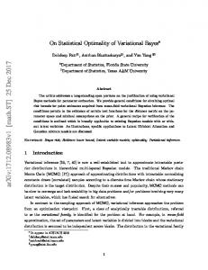
The data in this application comprise a set of soil phosphate measurements taken during the 1987 year of the Laconia Archaeological Survey in Greece. Soil phosphate concentration, resulting from the decomposition of organic material, is often higher in areas where archaeological activity is known to have taken place. Therefore, locating regions of high and low phosphorus content across a survey area can be helpful in identifying sites where archaeological activity has occurred. The measurements in this dataset were taken over a 16 by 16 grid at 10m intervals at the Greek archaeological site and there are missing data at 9 of the sites. These data were first analysed by Buck et al. (1988), using Bayesian change-point analysis, and later by Besag et al. (1991) using Bayesian image analysis techniques with an Ising model representation. We model the data using the Ising model and we assume that the means and variances of the Gaussian noise distributions are unknown and estimate them along with the association parameter β. Following the previous analyses, we assume Gaussian distributions for the log phosphate concentrations in mgP/100g of soil. However, unlike the previous analyses of the data we do not assume equal variances for the noise models. We used the same uninformative priors for the means and precisions as in the previous section. Table 3 displays the posterior means resulting from four different analyses of this dataset. The first two methods are the variational approach presented in this paper using the PL approach and the RDA approach conditioning on 10 rows (no advantage was achieved by conditioning on more than 10 rows) to estimate the normalising constant. Results are also given from two MCMC analyses of the data using the forward recursion method and the auxiliary variable MCMC method, respectively, for comparison. Figures 1 and 2 represent the areas which were identified as being high or low in phosphorous concentration. In these figures the posterior probability of high concentration at each grid site is plotted using a grey scale in which high concentration corresponds to black and low concentration corresponds to white. [TABLE 3 ABOUT HERE] We used a uniform prior for β over the range 0 to 0.6. The PL approximation has led to 20
an overly high estimate of β. This is apparent in Figure 1 as the evidence of human presence in the lower right section of the grid is suppressed and the map of high and low areas we obtained when using the PL shows less similarity to that obtained using the other methods. The Gibbs sampling analysis of this dataset based on the PL of Besag et al. (1991) also resulted in an overly high final estimate β. However, despite the overestimation of β that is obtained from the PL approach, we can see from Table 3 that the resulting variational posterior parameter estimates still compare favourably with those of the other analyses. The estimates of β resulting from the variational Bayes with RDA approach, the auxiliary variable MCMC method and recursive method are in close agreement. The regions identified by variational Bayes with the RDA approximation as having high posterior probability of human archaeological activity (Figure 2) are comparable to those found by an auxiliary variable MCMC analysis, by the recursive method and those found in Besag et al. (1991). All of these methods find two main activity areas and a smaller area in the lower right part of the grid. The analysis by Buck et al. (1988) did not provide posterior probabilities for the phosphorous concentration levels, but it also picked out two larger regions of likely activity and one smaller area. The computing time required to perform both variational analyses was considerably shorter than that needed for the recursive and auxiliary variable approaches. On a 3.2Ghz Pentium 4 desktop pc with 1 GB of RAM, the computing time for the recursive analysis was approximately 3 days and the time taken for the auxiliary variable analysis was approximately 24 hours while variational Bayes with PL took approximately 5 minutes and variational Bayes with RDA took around 7 minutes. [ FIGURE 1 ABOUT HERE ] [ FIGURE 2 ABOUT HERE ]
21
6
Conclusions
We have shown how a variational Bayes scheme can be constructed to analyse a hidden Potts model and demonstrated the results on binary images. In doing so we have demonstrated that variational Bayes is an effective means of inference in the challenging situation where noise model parameters and the association parameter in the Gibbsian model are unknown. We have also compared the quality of results obtained when using two alternative approaches to overcome the normalising constant estimation problem. Both approaches resulted in a time efficient algorithm and good approximations to the noise model parameters. However, the use of the RDA to approximate the normalising constant led to more accurate results on the whole than did the PL approach. In addition, we compared the variational scheme with two recent MCMC approaches in our analysis of a real data set and synthetic datasets. The computational time for the variational analyses was significantly shorter than that required for the MCMC analyses. Results from the variational Bayes analysis were comparable with the MCMC results lending further support to the usefulness of variational approximate methods for HMRF inference in the particular case where the Ising model is used to represent the data. Extension of the variational Bayes technique to more general HMRF-type models such as the autologistic model is possible and is a topic of current research. The variational technique can be straightforwardly applied to models belonging to the exponential-family therefore we can easily replace the noise model with another from that family. Using a secondorder neighbourhood structure would not excessively increase the computation time for a variational analysis therefore future work will include investigation of what improvements in inference the use of a higher order neighbourhood might bring.
Appendix To derive the variational posterior distributions we have to maximise the lower bound (1). We can express the lower bound as follows.
22
Z X
q(θ, z) log
{z}
=
Z X
( qz (z)
K Y
p(y, z, θ) dθ q(θ, z) ) ql (φl ) qβ (β) log
{
Qn QK i=1
l=1
{z}
Q p(yi |φl )zil }p(z|β){ K p(φl )}p(β) nQ o l=1 dφdβ K qz (z) q (φ ) q (β) l β l=1 l
l=1
(13) To find the form of the posterior for qz (z) we concentrate on the parts of (13) that involve z to obtain the following: Z X
( qz (z)
{z}
=
X
qz (z) log
)
Q Q zil { ni=1 K l=1 p(yi |φl ) }p(z|β) ql (φl ) qβ (β) log dφdβ qz (z) l=1
K Y
exp
+ terms not involving qz (z) o o Pn PK l=1 ql (φl ) qβ (β) i=1 l=1 zil log p(yi |φl ) + log p(z|β)dφdβ
nR nQ K
qz (z)
{z}
=
X
qz (z) log
exp
nP
n i=1
+ terms not involving qz (z)
o l=1 zil Eφl log p(yi |φl ) + Eβ log p(z|β)
PK
qz (z)
{z}
+ terms not involving qz (z) . The above expression is optimised when K n X X zil Eφl log p(yi |φl ) + Eβ log p(z|β)}. qz (z) ∝ exp{ i=1 l=1
Similarly, to optimise qφ (φ), we concentrate on the parts of (13) that involve φ as follows.
23
Z X
( qz (z)
=
) ql (φl ) log
{
Qn QK i=1
l=1
{z}
Z (Y K
K Y
) ql (φl ) log
{
Q p(yi |φl )zil }{ K l=1 nQ o l=1 K l=1 ql (φl )
p(φl )}
dφ
+ terms not involving qφ (φ) Q p(yi |φl )qil }{ K p(φl )} l=1 nQ o l=1 dφ K q (φ ) l l l=1
Qn QK i=1
l=1
+ terms not involving qφ (φ) . This expression is maximised when ql (φl ) ∝
n Y
{p(yi |φl )qil } p(φl ).
i=1
Similarly, to optimise with respect to qβ (β), we obtain that (13) is Z X Z =
qz (z)qβ (β) log
{z}
qβ (β) log
p(z|β)p(β) dβ qβ (β)
+
exp{Ez log p(z|β)}p(β) dβ qβ (β)
terms not involving qβ (β) +
terms not involving qβ (β) .
Thus, the optimal qβ (β) is qβ (β) ∝ exp{Ez log p(z|β)}p(β).
Acknowledgements The authors would like to thank the assistant editor and two anonymous reviewers for their constructive suggestions which led to improvements in this paper. The research of the authors CAM, RR and ANP was partially supported by an Australian Research Council Grant DP0558199. 24
References Attias, H. 1999. Inferring parameters and structure of latent variable models by variational Bayes. In: Proceedings of 15th Conference on Uncertainty in Artificial Intelligence. Beal, M.J. and Gharamani, Z. (2003). The variational Bayesian EM algorithm for incomplete data: with application to scoring graphical model structures. In: J.M. Bernardo, M.J. Bayarri, J.O. Berger, A.P. David, D. Heckerman, A.F.M. Smith and M.West. (Eds), Bayesian Statistics 7: Proceedings of the Seventh Valencia International Meeting (Oxford University Press), pp. 453-464. Besag, J. 1974. Spatial interaction and the statistical analysis of lattice systems (with discussion). Journal of the Royal Statistical Society, Series B 36: 192-236. Besag, J. 1975. Statistical analysis of non-lattice data. The Statistician 24: 179-195. Besag, J. 1986. On the statistical analysis of dirty pictures (with discussion). Journal of the Royal Statistical Society, Series B 48: 259-302. Besag, J., York, J. and Mollie, A. 1991. Bayesian image restoration, with two applications in spatial statistics (with discussion). Annals of the Institute of Statistical Mathematics 43: 1-59. Besag, J. and Higdon, D. 1999. Bayesian analysis of agricultural field experiments. Journal of the Royal Statistical Society, Series B 61: 691-746. Buck, C.E., Cavanagh, W.G. and Litton, C.D. 1988. The spatial analysis of site phosphate data, Computer Applications and Quantitive Methods in Archaeology. British Archaeological Reports, International Series, 446, eds. S.P.Q. Rhatz Corduneanu, A. and Bishop, C.M. 2001. Variational Bayesian model selection for mixture distributions. In: T. Jaakkola and T. Richardson (Eds), Artificial Intelligence and Statistics (Morgan Kaufmann), pp. 27-34.
25
Friel, N., Pettitt, A.N., Reeves, R. and Wit, E. 2006. Bayesian inference in hidden Markov random fields for binary data defined on large lattices. Submitted for publication. Gelman, A. and Meng, X.L. 1998. Simulating normalizing constants: from importance sampling to bridge sampling to path sampling. Statistical Science 13: 163-185. Geman, S. and Geman, D. 1984. Stochastic relaxation, Gibbs distributions, and the Bayesian restoration of images. IEEE Transactions on Pattern Analysis and Machine Intelligence 6: 721-741. Gottardo, R., Besag, J., Stephens, M. and Murua, A. 2006. Probabilistic segmentation and intensity estimation for microarray images. Biostatistics 7: 85-89. Green, P.J. and Richardson, S. 2002. Hidden Markov models and disease mapping. Journal of the American Statististical Association 97: 1055-1070. Jordan, M. 2004. Graphical models. Statistical Science 19: 140-155. MacKay, D.J.C. 1997. Ensemble learning for hidden Markov models. Technical Report, Cavendish Laboratory, University of Cambridge. McGrory, C.A. 2005. Variational Approximations in Bayesian Model Selection. PhD Thesis, University of Glasgow, UK. McGrory, C.A. and Titterington, D.M. 2006a. Variational approximations in Bayesian model selection for finite mixture distributions. Computational Statistics and Data Analysis, to appear. McGrory, C.A. and Titterington, D.M. 2006b. Bayesian analysis of hidden Markov models using variational approximations. Submitted for publication. Møller, J., Pettitt, A.N., Reeves, R. and Berthelsen, K.K. 2006. An efficient Markov chain Monte Carlo method for distributions with intractable normalising constants. Biometrika 93: 451-458.
26
Murray, I., Ghahramani, Z. and MacKay, D.J.C. 2006. MCMC for doubly-intractable distributions. Preprint. Newman, M.E.J. and Barkema, G.T. 1999. Monte Carlo Methods in Statistical Physics. Oxford University Press. Pettitt, A.N., Friel, N. and Reeves, R. 2003. Efficient calculation of the normalising constant of the autologistic and related models on the cylinder and lattice. Journal of the Royal Statistical Society, Series B 65: 235-247. Reeves, R. and Pettitt, A.N. 2004. Efficient recursions for general factorisable models. Biometrika 91: 751-757. Ryd´en, T. and Titterington, D.M. 1998. Computational Bayesian analysis of hidden Markov models. Journal of Computational and Graphical Statistics 7: 194-211. Smith, M. and Fahrmeir, L. 2006. Spatial Bayesian variable selection with application to functional magnetic resonance imaging, Journal of the American Statististical Association. To appear.
27
List of Figures
Fig. 1. High and low phosphorous areas as identified by variational Bayes with PL estimation Fig. 2. High and low phosphorous areas as identified by variational Bayes with RDA
28
Table 1: Estimation of parameters in the simulation study using the variational Bayes scheme: averages from 20 replications True Distribution
Variational Post. Means using PL µˆ1 σˆ1 βˆ µˆ2 σˆ2
Variational Post. Means using RDA 10 µˆ1 σˆ1 βˆ µˆ2 σˆ2
βˆ
µˆ1 µˆ2
σˆ1 σˆ2
0.30
−1.00 1.00
0.60 0.60
0.315
−0.998 1.010
0.598 0.599
0.300
−0.999 1.001
0.596 0.598
0.30
−1.00 1.00
0.70 0.70
0.331
−1.050 0.989
0.669 0.731
0.303
−1.042 0.985
0.697 0.711
0.30
−1.00 1.00
1.00 1.00
0.389
−1.044 0.899
0.985 1.044
0.288
−1.032 1.014
0.936 0.938
0.30
−1.00 1.00
1.25 1.25
0.424
−1.117 0.882
1.326 1.295
0.269
−1.105 1.126
1.085 1.116
0.40
−1.00 1.00
0.60 0.60
0.412
−1.005 1.007
0.596 0.587
0.400
−1.002 1.001
0.597 0.596
0.40
−1.00 1.00
0.70 0.70
0.439
−0.981 1.081
0.730 0.679
0.403
−0.987 1.124
0.678 0.727
0.40
−1.00 1.00
1.00 1.00
0.445
−0.958 1.120
1.010 0.978
0.398
−0.975 1.122
0.967 0.972
0.40
−1.00 1.00
1.25 1.25
0.491
−0.902 1.288
1.289 1.255
0.391
−0.980 1.047
1.185 1.192
29
Table 2: Estimation of parameters in the simulation study using the auxiliary variable method: averages from 20 replications True Distribution
Post. Mean using auxiliary variable MCMC µˆ1 σˆ1 βˆ µˆ2 σˆ2
βˆ
µˆ1 µˆ2
σˆ1 σˆ2
0.30
−1.00 1.00
0.60 0.60
0.297
−1.010 0.997
0.594 0.597
0.30
−1.00 1.00
0.70 0.70
0.298
−1.012 0.995
0.693 0.696
0.30
−1.00 1.00
1.00 1.00
0.299
−1.013 1.000
0.989 0.991
0.30
−1.00 1.00
1.25 1.25
0.299
−1.014 1.003
1.233 1.288
0.40
−1.00 1.00
0.60 0.60
0.399
−1.007 0.984
0.594 0.603
0.40
−1 1
0.70 0.70
0.398
−1.009 0.982
0.693 0.702
0.40
−1 1
1.00 1.00
0.399
−1.012 0.977
0.986 0.999
0.40
−1 1
1.25 1.25
0.403
−1.036 0.963
1.233 1.253
30
Table 3: Estimates of model parameters resulting from alternative analyses of the soil phosphate dataset Variational Post. Variational Post. Means using PL Means using RDA 10 βˆ µ ˆ1 σ ˆ1 µ ˆ2 σ ˆ2
0.599 3.871 0.345 4.349 0.278
0.445 3.851 0.337 4.349 0.275
31
Recursive Method Post. Means
Auxiliary Variable MCMC Post. Means
0.442 3.897 0.361 4.360 0.239
0.442 3.895 0.359 4.359 0.241