This procedure, which we call static load balancing, has been standard for all TWOS. performance .... messages sent to this object from the start of the simulation up to, but not including, .... The TWOS dynamic load management facility requires.
VIRTUAL TIME BASED DYNAMIC LOAD MANAGEMENT IN THE TIME WARP OPERATING SYSTEM Peter L. Reiher Jet Propulsion Laboratory 4800 Oak Grove Drive Pasadena, CA 91109-8099 David Jefferson Department of Computer Science University of California, Los Angeles Los Angeles, CA 90024 Keywords: Time Warp, dynamic load management, parallel operating systems, parallel and distributed simulation, optimistic synchronization Abstract The Time Warp Operating System (TWOS) executes event-driven simulations in an optimistic style on parallel machines. Recently TWOS has been substantially improved by the addition of dynamic load management for the purpose of (a) handling fluctuations in a simulation’s performance, (b) dealing effectively with dynamic creation and destruction of processes, and (c) eliminating the burden on users of assigning processes to processors. Because TWOS uses optimistic synchronization, existing load management theory, which tends to be based on balancing processor utilization, is not applicable; TWOS instead balances load using a more general metric called effective utilization. In addition, TWOS introduces a new program unit called a phase, which is a process delimited by two simulation times. In TWOS, the phase, not the process, is the fundamental unit of scheduling, migration, and rollback, as well as the target of messages. This paper describes early results of our experiments with the TWOS dynamic load management facility. It covers the theory and mechanics of phase splitting and migration, and presents performance results for several combinations of benchmark, configuration, and load management policy. 1. Introduction The Time Warp Operating System (TWOS) is a virtual time-based operating system that runs event-driven simulations on parallel processors (Jefferson 1987). It has been built over the last several years at the Jet Propulsion Laboratory, and runs primarily on the BBN Butterfly GP1000 under Chrysalis. It executes simulations optimistically using
the Time Warp mechanism, so that not all of its work is guaranteed to be entirely correct at first; it assumes its work is correct until contrary evidence appears, at which point the incorrect part of the computation is rolled back and re-executed correctly. Dynamic load management is a different problem in TWOS than in most distributed systems. First, TWOS runs a single multiprocess job at a time, with the goal of completing that job as quickly as possible. TWOS’ load management facility tries to meet that goal, rather than trying to maximize utilization of the hardware. Second, because TWOS operates optimistically, unlike other operating systems, it does not block processes at synchronization points; it simply executes them ahead optimistically. Hence, it rarely leaves its processors actually idle; the work they do may be rolled back later, but they are only rarely without any work to do at all. TWOS’ reliance on virtual time offers several load management possibilities not available in other systems. TWOS simulations are decomposed into objects representing parts of the simulated system. This division is referred to as spatial decomposition. The use of virtual time permits objects to be further divided temporally into units called phases. A phase is a portion of the execution of an object that is delimited by two virtual times. For example, phase A[100..200) is the execution of object A from simulation time 100 up to (but not including) 200. In TWOS the phase is the fundamental unit of computation, not the object. They are the units of scheduling, rollback, and migration, and the targets of messages. Unlike decomposition into objects, which must be done by the simulation programmer, the decomposition into phases can be done automatically at run time as part of load management policy. In the absence of dynamic load management, the user must find a static assignment of objects to processors that produces an approximately balanced workload when integrated over the entire execution. This is not an easy task; without performance information, the best that can be done is to assign an equal number of objects to each processor and hope that the total workload per processor will be approximately even. Except in special circumstances this will be highly unlikely, and a large amount of processor time will be lost, especially when there are few objects per processor. A better approach is to run the application once to obtain timing data indicating how much of the work was done by each process. A bin packing algorithm can then be used to find an assignment which gives nearly the same amount of work to each processor. This procedure, which we call static load balancing, has been standard for all TWOS performance studies, and generally produces much better performance than simply balancing the number of objects. But static load balancing is not foolproof, and can yield terrible performance. As an extreme case, suppose a simulation is composed of four objects, A1, A2, B1, and B2. All four use the same amount of processor time, but at the beginning of the simulation A1 and A2 do all of the work, while at the end B1 and B2 do all of the work. On a two-processor machine any configuration in which there
are two objects per processor is “balanced”. But pairing (A1,B1) on one processor with (A2,B2) on the other will execute with full 2-fold parallelism for the entire execution and will run twice as fast as the pairing (A1,A2) and (B1,B2) in which there is no parallelism at all. Of the three “balanced” configurations, two are good and one is terrible. Dynamic load management would correct this problem at run time. Even when static load balancing does produce good runtime performance it has one profound flaw: it requires that the simulation be run once, slowly, just to get the performance information needed to decide how to configure it so it runs quickly. On the face of it, this is a ridiculous procedure. Static load balancing can only be effective if the same simulation will be run many times with varying parameters and random seeds and most runs have similar performance dynamics as the single run made to gather the performance data. In that case a single static assignment will work well for all of the runs. Sometimes this is the case, and sometimes not, but the only way to find out is to try a new static assignment. Finally we should note that static load balancing is very brittle. A small change in the hardware configuration can make a large change in the optimal static configuration and force a recalculation of the assignment. Any change in the number of processors, or the amount of memory, or in the I/O configuration and its attendant interrupt traffic, could spoil a previously good assignment of objects. Similarly, small changes in the software of either the TWOS system itself or the simulation can radically change the optimal static configuration. For these reasons, the primary goal of TWOS’ dynamic load management is to allow the system to perform well without static load balancing, using a much less carefully balanced initial assignment, particularly on jobs that run a long time. While a good static assignment might make a job reach a good balance more quickly, it might not, and in any case dynamic load management permits less effort in producing the initial static assignment. A second goal is to perform well in the face of dynamic creation and destruction of objects. When an object is dynamically created in a parallel system, some form of dynamic load management is needed to ensure a good assignment of the new object to a processor. Without system support, either the user must assign the new object’s location himself (which makes the code non-portable), or he must rely on the default assignment. Dynamic object destruction causes a similar need. If an object is destroyed without redistributing the load, the system is likely to become unbalanced because of the lost workload. The final goal of TWOS’ dynamic load management is to provide additional speedup beyond what can be achieved with a static assignment. Currently, TWOS simulations sometimes achieve within 30% of the critical path speedup, so dynamic load management may not always have sufficient additional speedup possible to allow it to
make up its costs. But substantial speedup is still available for many simulations, and dynamic load management may be able to extract some of it. TWOS load management strategy is committed to transparency. The user is never required to offer advice or validate the decisions of the system’s dynamic load manager. Nor should the user need to encode load management advice into the application program. TWOS takes complete responsibility for all dynamic load management decisions. This paper describes the implementation of dynamic load management for TWOS. This implementation is not suitable for parallel processors with many more than 100 nodes. A future version of the dynamic load management system is expected to scale better. Also, the system does not include a number of potential performance improving features, and has not been fully tuned for a wide variety of applications. However, this implementation achieves most of the goals set for TWOS dynamic load management, including improved performance for many important cases. Performance results are included in this paper. The final implementation is expected to achieve even better performance over a wider range of applications. 2. The Time Warp Operating System A TWOS simulation is divided into objects that communicate via event messages. An arriving message causes an object to perform an event. TWOS takes care of message delivery, scheduling, resource management, and synchronization. A more complete description of TWOS can be found in (Jefferson 1987). TWOS currently runs on the BBN Butterfly Plus parallel processor. Synchronization in TWOS is achieved by an unusual mechanism based on the concept of virtual time (Jefferson 1985 and Jefferson 1987). Each message is tagged with a virtual time, indicating the order within the simulation in which the messages are to be processed. TWOS produces the same effect as processing all messages strictly in timestamp order, though the system might actually handle them in a different order. TWOS objects are composed of one or more phases. Each phase has responsibility for handling all of an object’s business for one interval of virtual time. Phases are the basic unit of scheduling in TWOS. Any phase can be located on any node in the distributed system, without regard for the location of the other phases of the same object. The system ensures that each message is routed to the node hosting the phase of the object that should handle it. Figure 1 shows an object named A divided into two phases. Each entity in this figure represents one phase. Each phase has a control block, an input queue of incoming messages, an output queue containing copies of outgoing messages, and a queue of saved states. The first phase runs from virtual times –_ to 1700, meaning that any
messages sent to this object from the start of the simulation up to, but not including, virtual time 1700 are handled by this phase. The second phase covers virtual times 1700 to +_, so any messages sent to the object from virtual time 1700 to the end of the simulation are handled by this phase. Phases are produced by temporal splitting. Temporal splitting allows any simulation object to be divided into two phases. Further temporal splits can divide objects into more phases. Temporal splitting can be invoked either at the beginning or in the middle of a run. An object can be split into an arbitrary number of phases, and each phase can be located on or migrated to a different node. When they are on different nodes, two phases of the same process can actually execute in parallel. Each node in a parallel processor running TWOS keeps a separate queue of phases to be run. Phases run when they receive messages. The state of the phase produced by handling the previous (in virtual time) message is used as input for running the next message. Scheduling is performed on a per-node basis by preemptive lowest virtual time first, across all phases on the node. On other nodes, messages with lower or higher virtual timestamps may be chosen, since each node schedules solely on local information. Whenever a Time Warp phase sends a message, the receiving object name and the virtual receive time are stamped on the message. TWOS uses this information to route the message not just to the correct object, but to the correct phase. Since any phase may send a message to any other phase, except those in the past, a phase on a node that is running far behind other nodes in virtual time may send a message to a phase on a node that is running far ahead. If the receiving phase has already run an event at a virtual time later than the sending phase’s message, the receiving phase must roll back. The receiving phase must restore its state to the virtual time before the arrival of the sending phase’s message and handle that message. If the receiving phase erroneously sent messages, they must be cancelled. Messages are cancelled in TWOS by sending antimessages. TWOS maintains sufficient information about past states of phases and the messages they sent to correctly handle any possible rollback. The use of phases has some costs. One is state duplication. In the temporally split object shown in figure 1, note that both phases store a state for virtual time 1500. This state is produced by the earlier phase’s input message at time 1500, and is the last state produced by that phase. Therefore, the later phase needs a copy of that last state as input for handling its first input message, at virtual time 1800. The state at time 1500 is shipped to the second phase for later use. Typical TWOS applications use states that are between a few hundred and a few thousand bytes in length, so the memory wasted due to the second copy of the state rarely exceeds 10K bytes. A second cost relates to rollback. Should the earlier phase’s message for virtual time 1500 be re-executed, with different results, the earlier phase must send a copy of the
new state for virtual time 1500 to the later phase, causing that phase to roll back and reexecute any work that depended on it. A rollback spanning two nodes is more expensive than a rollback confined to a single node. Despite these costs, temporal splitting allows great flexibility in dynamic load management. The dynamic load management system can use temporal splitting to predictively migrate phases, to limit the cost of migrating a phase, and to handle memory exhaustion problems during migrations. Many of these possibilities have not been explored yet, but sufficient evidence exists for the value of phases even without these options. 3. Related Work Load management research has a long history. Much of this research was based on assumptions that do not apply to TWOS, or had goals different from those of TWOS. Dynamic load management is typically either load balancing or load sharing (Hailperin 1985). Load balancing tries to equalize some metric, typically utilization, across all nodes, usually by migrating existing objects. Load sharing usually involves spawning new processes on idle nodes. Load balancing is only possible in systems that can migrate already running processes (Li 1988). TWOS recognizes the need to assign new objects to nodes in accordance with load criteria, but also migrates existing objects to improve the performance of the system. Speed of completion of a single job is not the only goal for many load management systems. Fairness, ensuring that each of several independent jobs gets its share of the system’s attention, is often important (Krueger and Livny 1987). TWOS runs a single job at a time. Since the independent parts of that job need not be treated fairly, as long as the job completes as quickly as possible, TWOS does not concern itself with fairness. Many algorithms have been proposed for moving load from one node to another, given that dynamic load management is being used. These include distributed drafting (Ni et al 1985), physics-based systems using gradient models (Lin and Keller 1986), and physics-based systems using simulated annealing or Hamiltonians (Fox 1986). While some of these methods offer suggestions on how to perform load management in TWOS, none solve the problem of managing load in a virtual time-based system. The KLOX operating system does address virtual time-based load management, but its goal is drastically different from the goal of TWOS (Chen 1988). KLOX investigates performance portability, rather than try to run applications as quickly as possible. Also, KLOX does not use optimistic synchronization. The Rand Corporation’s Time Warp system performs dynamic load management in a virtual time environment, even including rollback, but again, their goals are different from those of TWOS (Burdorf and Marti 1990). The Rand implementation of Time
Warp runs on a network of personal workstations, and tries to make use of idle cycles on machines on the network. Its extremely high granularity (multiple seconds per event) and the relatively slow local area network connection resulted in a very different performance environment than that of TWOS. Balancing load based on the utilization of nodes is 1985). However, optimistic systems need to balance rather than balancing the total work, which is what utilization. Since little research has been done on systems, this distinction has not arisen before.
a fairly common idea (Hailperin the amount of useful work done, is measured by simple processor load management for optimistic
Some form of object migration is needed if existing objects are to be shifted among the system’s nodes. Many existing distributed systems support process migration, including Accent (Zaya 1987), Locus (Popek and Walker 1985), Sprite (Douglas and Ousterhout 1987), DEMOS/MP (Miller 1987), the V kernel (Theimer et al 1985), KLOX (Li 1988), and the Rand Time Warp implementation (Burdorf and Marti 1990). Of these, only KLOX and Rand Time Warp have access to virtual time in their migration mechanism, and neither use the concept of temporal splitting to assist in migration. Most of the existing work on dynamic load management does not deal with virtual time systems. The work that does is for systems with different goals and, hence, different approaches to load management. Even these systems do not make any use of the concept of phases or use an appropriate load management metric. 4. TWOS Dynamic Load Management Tools Dynamic load management is performed in TWOS by moving phases from one node to another during the run. The goal of the load manager is to minimize the application’s real time to completion. The basic tools of TWOS’ dynamic load manager are temporal splitting and phase migration. Temporal splitting permits objects to be divided into smaller components. One phase of an object is much less expensive to migrate than the entire object because it has fewer states and messages. TWOS phase migration permits any phase to be migrated to any other node in one operation. The typical TWOS object, at a given point in the simulation, probably has several input messages saved, along with a number of saved states and negative copies of messages it has sent. Some of the input messages have already been processed, some have not. Associated with each saved item is a characteristic simulation time. For input messages, this time is the arrival time of the message. For states, it is the time at which the state was produced. For output messages, it is the time at which the message was sent.
The lengths of an object’s input, output, and state queue vary quite a lot, depending on the characteristics of the particular simulation, the assignment of objects to nodes, and the current state of the simulation. Some typical lengths of these queues are 2 for the state queue and around 4 for both of the message queues. The maximum sizes during a run can be much larger, though. All three queues have been seen grow to over 100 entries each, and have no set maximum length, other than limitations of the total amount of memory available on a node. If all of the queues’ data had to be moved on every migration, some migrations could take a very long time to complete. The value of completing a process migration as soon as is practical is widely recognized (Zaya 87), so permitting the migration of objects with a lot of data in their queues must be avoided. However, such objects may be precisely those that are most desirable to migrate, for load management purposes. Temporal splitting solves this problem. Temporal splitting permits TWOS to dynamically divide any object into two phases. These phases may be further subdivided into smaller phases by subsequent splits. Each phase has responsibility for handling all of the object’s activities during a certain period of simulation time. Object migration in TWOS is actually phase migration. The phase migration mechanism permits the migrating phase to run as soon as sufficient information has moved to permit execution to begin. The remainder of the migration will continue in the background. Phases of any size, including complete objects, can be migrated. The TWOS load management facility requires no special assumptions about system performance. TWOS already required reasonable delivery times for messages in order to achieve good performance. The TWOS dynamic load management facility requires the same general speed of delivery. Beyond that, it takes responsibility for ensuring that migrations complete in reasonable times. The dynamic load management facility also assumes that object states and messages are much smaller than the amount of memory available on a node. TWOS already required that assumption, as the system is required to keep many messages and states in memory simultaneously. Finally, the current TWOS load management facility assumes that only the data for a phase need be moved, not the code. However, the existing system already kept all code for all object types on all nodes. One possible load management policy is to make all nodes progress in virtual time at more or less the same rate, with respect to real time. Hence we measure “load” by virtual time: high virtual time is interpreted as low load, and vice-versa. Nodes far behind in virtual time would migrate phases to nodes far ahead. Since the TWOS scheduler favors earlier virtual times, the phases that were far behind will be scheduled more often on the nodes that were running far ahead. As a result of the migrations, lagging nodes will probably schedule work for later virtual times than they would have
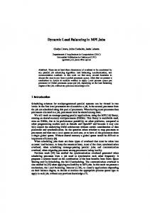
without the migrations. The ahead nodes will schedule earlier work, the behind nodes will schedule later work, so presumably the set of nodes would show less spread in the virtual times being worked on. The problem with this choice of load metric is that virtual time encodes synchronization constraints, not relative amounts of processor time necessary to progress from event to event. Figure 2 illustrates the problem. The two vertical scales indicate progress in the simulation in virtual time and processor cycles. Each mark on a scale indicates a set of events. On the virtual time scale, the events happen at the indicated virtual time. The greater the distance between two marks on the processor cycles scale, the more cycles were required to complete the events. Arrows connect corresponding marks on the virtual time and processor cycle scales, indicating when events occurred on those two scales. In this example, handling the events at virtual time 100 takes much less processor time than handling the events at virtual time 200. In each case, from a virtual time point of view, completing the events at those virtual times permits the application to advance 100 virtual time units. Therefore, if the goal of the dynamic load manager was related to the rate of progress of virtual time, the load manager should devote equal attention to progressing from virtual time 100 to virtual time 200 as it does in progressing from virtual time 200 to virtual time 300. However, since many more processor cycles must be expended to get past virtual time 200, the dynamic load manager will do better to exert more effort in making this part of the application progress than in making the events at virtual time 100 go faster. The load manager should be more willing to migrate phases in response to the load resulting from events at time 200 than those at time 100. In actuality, what should be balanced is not the spread of virtual times, but the proportion of useful processor cycles being spent. Generally speaking, some work done in a TWOS run will be rolled back, and some will not. The work that will not be rolled back is called effective work. The fraction of work on a given node that is effective is the node’s effective utilization. A node with a high effective utilization is contributing a lot to the computation, while one with low effective utilization is contributing comparatively little. The effective utilization theory implies that the system should try to shift load off nodes doing a lot of effective work and onto nodes doing little effective work. Effective utilization is the analog in optimistic systems for simple node utilization in other systems (Hailperin 1985). In optimistic systems, simple node utilization is always high, since the system optimistically performs work that may need to be discarded later. In these systems, balancing the work that does not need to be discarded is the analog to simple utilization, and balancing on effective utilization has precisely that effect.
Balancing on the basis of effective utilization is better than balancing on the rate of progress of virtual time because the former is invariant in the face of order-preserving virtual time relabeling, while the latter is not. Consider two applications that are absolutely identical, except that every event in the second has a different virtual timestamp than the corresponding event in the first. Exactly the same events, causing exactly the same sequences of instructions are performed in the two applications in exactly the same order. Only the virtual time labels on events and messages are different, but they are not uniformly different. A good set of migrations for the first application should be good for the second, as well. However, if decisions to migrate are based on which nodes are far ahead and far behind in virtual time, the different, non-linear labelings of virtual times may cause a vastly different set of migrations to be ordered for the second application. If the system balances on the basis of effective utilization, since precisely the same instructions are being executed, the effective utilizations for the system will be the same, and the same set of migration decisions is likely to result. TWOS uses a dynamically calculated estimator of effective work to perform dynamic load management. Whether a given piece of work contributes to a phase’s effective work cannot be known with certainty until that piece of work is either discarded or committed. But a piece of work might not be committed until long after it was produced. Therefore, TWOS must use an estimator of effective work. This estimator is produced by keeping track of how much processor time was used for each event. That amount is added into the phase’s effective work estimator. One of two things will happen to the event. Either a rollback will occur for that virtual time and the event will be discarded, or no rollback will occur and eventually the event will be committed. In the latter case, the optimistic assumption that good work was done to produce the event was justified, so the phase’s effective work estimator need not be adjusted. If the event is discarded due to rollback, however, then the amount of work required to run it must be subtracted from the phase’s effective work estimator. When the load manager needs to determine if a given node is overloaded or underloaded, it must determine that node’s effective utilization, which is the fraction of time that it spends doing effective work. Overhead does not count as effective work, nor does work that has been rolled back, so the effective work of a node is the sum of the effective work measurements for all phases on that node. Since TWOS only produces an estimator of each phase’s effective work, it can produce only an estimator of each node’s effective utilization. Assuming that the behavior of objects is fairly smooth over longer intervals than one effective utilization computation interval, the estimator should be fairly accurate. Load management cycles are started by one node. Periodically, this node sends the initialization messages for an effective utilization gathering protocol. This protocol imposes a graph structure on the nodes of the system like that used by TWOS’ current
global virtual time algorithm, which is used for commitment purposes (Bellenot 90). Every node receives information from either one or two other nodes, and sends information to either one or two other nodes. The incoming information is a table of all effective utilizations so far collected by the protocol. Once a node has received all of its incoming messages and merged their tables of data, it calculates its own current effective utilization and adds it to the merged table, which is then sent on to one or two other nodes. When the node at the terminus of the graph receives the complete table, it sends it back in the reverse direction, along the same graph. Each node, upon receipt of the complete table, examines it to determine if it is one of the most overloaded nodes in the system. If so, it matches itself to one of the underloaded nodes. The most overloaded node matches to the most underloaded, the second highest load matches to the second lowest, and so on. Only nodes whose effective utilization differ by some threshold amount will actually perform migrations. Overloaded nodes select a good phase to migrate. Informally, the chosen phase should minimize the difference in effective utilizations of the overloaded and underloaded nodes. More formally, if overloaded node m and underloaded node n are paired, m has utilization um and n has utilization un. m must try to find a phase to migrate to n. (For simplicity, assume that only a single phase, at most, will be moved. In actual practice, moving several phases may be better.) m should try to choose a phase p such that it minimizes |(um – up) – (un + up)| In some cases, m may not be able to find a phase to migrate that will bring the two nodes’ effective utilizations any closer together. In such cases, nothing should be moved. This method of choosing phases to migrate uses certain assumptions. An important one is that migrating a phase from a node with high effective utilization (m) to a node with low effective utilization (n) will cause n to run the migrated phase often enough to actually improve its effective utilization. While not necessarily true, experience with the load management facility shows that this assumption is usually valid. A second important assumption is that the effective work moved off m will be replaced, at least in part, by some other effective work. If not, effective utilization is merely being shuffled around to no purpose. Put more formally, the expectation is that, after the migration, the effective utilizations of nodes m and n for the next load management cycle, um’ and un’ will be greater than um and un, or um’ + un’ > um + un
Were this assumption false, load management would not improve performance, since the migration would cause no improvement in the total amount of effective work done by the nodes. Actual performance results demonstrate that the above formula usually holds. Once a phase has tentatively been chosen as a candidate for migration, m splits the chosen phase into two smaller phases. This split limits the amount of data that must be migrated. The resulting phase covering the later interval is then migrated. Node n thus gets the virtual future portion of the split phase, which is usually the part that will do the most work in the real time future. 5. Performance Results The TWOS dynamic load management facility has been applied to all of the major applications currently run under TWOS. This section presents performance results for some of those applications. The TWOS dynamic load management facility is functional, but has not been fully tuned. It has several load management parameters that can be set to vary the way load management proceeds, and the best settings, or methods for setting these parameters, have not yet been determined. One important parameter is the value of the threshold difference between an overloaded node’s and an underloaded node’s utilizations that is necessary to cause them to perform a migration. For high utilization um and low utilization un, and threshold t, the inequality um - un ³ t must hold in order to perform a migration from m to n. Effective utilizations typically have values between 0 and 1. Under some circumstances, an effective utilization can be negative, due to sudden rollback of all work performed during several load management cycles. Effective utilization can never be greater than 1. Unless otherwise indicated, the threshold utilization difference for all measurements shown here is .1. The length of time between dynamic load management cycles is another parameter that can have a dramatic effect on performance. The default time for load management cycles is 4 seconds. The minimum permitted cycle time is 2 seconds. There is no maximum permitted cycle time, though cycle times on the order of the application’s run time will clearly prevent dynamic load management from doing much. The number of pairs of nodes that can order migrations during each cycle is also controlled by a parameter. The default value for this parameter in these performance
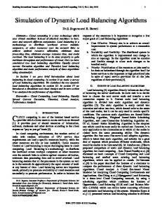
results is 1, meaning only the most utilized and least utilized nodes are eligible for migration during a cycle. The method used for splitting objects selected for migration can be varied. The default method is to split at the virtual time of the last event the object ran. Other methods are to split at the latest virtual time of any item in an object’s queues, or not to split at all. Section 5.1 presents results for three applications under the default parameter settings. Section 5.2 then shows the effects of varying the dynamic load management parameters for a single application. Section 5.3 discusses the amount of data moved during a migration and the typical latency of migrations. Section 5.4 shows how dynamic load management gradually evens out the effective utilizations of various nodes in a run. The speedups shown in section 5.1 are relative to running a sequential simulator on a single node of the same machine used for the TWOS runs. The sequential simulator uses a splay tree for its event queue. It never performs rollback, and hence has a lower overhead than TWOS. The sequential simulator links with exactly the same application code as TWOS. It is intended to be the fastest possible general purpose discrete event simulator that can handle the same application code as TWOS. In all cases, the points plotted represent the average of four identical runs of TWOS. Without dynamic load management, there is typically little variation in the run times. Using dynamic load management introduces much more variation. The resolution of measurement is 3 seconds for run times and resulting speedups. 5.1 Basic Dynamic Load Management Performance Figures 3, 4, and 5 show the performance of TWOS with dynamic load management compared to its performance without dynamic load management for three different applications. The first application is STB88, a simulation of theater level combat (Wieland 89). The second application is pucks, a simulation of frictionless twodimensional pucks moving and colliding on a table (Hontalas 89). The third application is WarpNet, a simulation of message passing in a packet switching network (Presley 89). The curves in this section plot points for numbers of nodes between 8 and 64 nodes. Every even multiple of 4 nodes is plotted. Figure 3 shows the results of using dynamic load management for STB88. The four curves in this figure represent running the simulation on varying numbers of nodes using two different initial configurations, with dynamic load management turned off and turned on. One configuration is carefully balanced. This configuration requires extensive work to produce, and must be re-done whenever the simulation is changed in any way. The other configuration used is simple to produce, and is probably the best configuration that a user not knowledgeable about parallel processing would typically
produce. This configuration simply assigns objects to nodes in a round-robin fashion, resulting in an equal number of objects on each node. The first type of configuration is referred to as a balanced configuration, while the second is called a realistic configuration. The quantity plotted in this figure is speedup, so higher points are better. The sequential simulator time for this application is 3672 seconds. For this application, dynamic load management is expected to perform well. STB88 is known to contain a major phase change in its behavior. In the first third of the simulation, most activity is units moving across the battlefield. In the remaining two thirds of the simulation, most activity is combat. Static load balancing tends to favor a balance that is good for the combat, at the cost of a good balance for the movement stage. The dynamic load management facility typically moves many objects during the early movement stage, but few in the later stage. Thus, dynamic load management has the potential to speed up this application by balancing the early, shorter stage. Examining the four curves in figure 3, the worst speedups come from running a realistic configuration file without using dynamic load management. This configuration file is simple enough for users to produce, but, as might be expected, is not well balanced for the overall simulation, and takes no account of the phase change in the simulation. No single curve similarly provides the best set of speedups for all numbers of nodes. Sometimes the balanced configurations without use of dynamic load management do best, sometimes the same configurations with dynamic load management are better. In one case, the best performance is obtained from the realistic configuration with dynamic load management applied. For numbers of nodes up to 40, the realistic configuration files with dynamic load management turned on do almost as well as the well-balanced configuration files without dynamic load management. At greater numbers of nodes, the well-balanced configurations begin to outstrip the realistic configurations with dynamic load management turned on. In these cases, the parameter settings used for the dynamic load management system may be restricting the speedup. In particular, as the number of nodes becomes larger, the ability of the dynamic load management system to correct imbalances by moving only a single object per load management cycle decreases. Comparing the two curves using the balanced configurations with and without dynamic load management shows a similar effect. Using dynamic load management matches or improves the speedup of the simulation up through 40 nodes. Beyond this point, dynamic load management actually slows the simulation down. Again, the restrictions on the dynamic load management system may explain why they did not speed the system up. The reason the system slowed down is probably because the migrations performed were insufficient to improve the performance, but got in the way of an otherwise good configuration. Starting at 44 nodes, the dynamic load management runs began to produce significantly more rollbacks than those without dynamic load management. For the two worst cases, 44 and 60 nodes, the dynamic
load management runs had around 50% more rollbacks than those without dynamic load management. Below 44 nodes, the dynamic load management runs usually had about the same number of rollbacks as the runs without it, or even significantly fewer. The average improvement in speedup for the realistic configuration files for dynamic load management was 19%. while the balanced configurations ran at precisely the same speed, on average, with or without dynamic load management. The biggest improvement in speedup was 32% for a realistic configuration, and 11% for a balanced configuration. The second application is pucks, a simulation of two-dimensional pucks moving and colliding on a frictionless surface bounded by cushions. This application can be run with many different configurations, varying the number of pucks on the table, the way the table surface is partitioned into objects, and the initial velocities and directions of the pucks’ movements. The particular configuration used in figure 4 simulates 128 pucks moving on a table divided into 8-by-16 sectors. The pucks are all moving along the major axis of the table, and never collide with each other. They move in a mass from one side of the table to the other, then collide with the cushions and reverse their direction. Figure 4 shows the resulting speedups from the pucks simulation using this configuration. Again, the four curves represent a realistic configuration and a static balance by amount of work done, with and without dynamic load management. The sequential simulator time for this pucks simulation is 6829 seconds. Perhaps the most interesting observation from this figure is that, unlike the curves for STB88, the balanced configurations do not always do better than the realistic configurations. This application has specific phase behavior, and a significant geometry in the problem. The static balancing only takes amount of computation into consideration, so more realistic configurations that happen to handle the geometry of the computation may do well. More to the point of this research, the dynamic load management points are almost all above the corresponding configuration without dynamic load management. Only at 36 nodes, for realistic configurations, did dynamic load management perform significantly worse. The performance improvements in the other cases were as high as 55% for realistic configurations, and 25% for balanced configurations. The average improvement for realistic configurations was 13%, and for balanced configurations 17%. For this application, dynamic load management applied to a realistic configuration outperforms a balanced configuration in almost all cases tested. Part of this effect is due to the fact that the realistic configuration often proved to be better than the balanced one, but dynamic load management applied to the realistic configuration
managed to beat the best configuration not using dynamic load management, in most cases. Dynamic load management is clearly improving the performance of pucks. Another interesting feature of figure 4 is that the curve for dynamic load management applied to realistic configurations is considerably smoother than the curve for the same configurations without dynamic load management. In certain cases, the realistic configuration was much worse than in others. Dynamic load management was largely able to smooth out the differences, however, resulting in more predictable speedup. Figure 5 shows the speedups for an application called WarpNet. WarpNet simulates message passing in a computer network. The nodes in the simulated network are not completely connected, so some messages must travel multiple hops to reach their destinations. Many different topologies can be simulated by WarpNet. The topology used in the set of runs shown in figure 5 contains 137 nodes connected in an irregular fashion, with an average of two to three links per node. The sequential simulator time for this warpnet simulation is 5485 seconds. WarpNet is not a good candidate for dynamic load management. Over a lengthy period, WarpNet usually achieves fairly steady behavior. Hot spots typically do not persist, so any work done by dynamic load management to overcome them is not likely to improve the run. Also, realistic configurations can perform quite well for WarpNet. None the less, figure 5 shows that dynamic load management is able to slightly improve the performance of the realistic configurations of WarpNet, in many cases. Only rarely does it do any worse. On the average, WarpNet using a realistic configuration file runs 3% faster with dynamic load management. Assuming a balanced configuration is used, warpnet runs at much the same speed with or without dynamic load management. Applying dynamic load management to a realistic configuration produces 5% less speedup than using a good static configuration, but, of course, saves the work of creating that static configuration. Thus, even for an application that is not well suited to dynamic load management, the TWOS dynamic load management system achieves reasonable performance. 5.2 Varying Dynamic Load Management Parameter Settings The remaining performance measurements examine the effects of varying several of the dynamic load management parameters. These remaining measurements are all for STB88. STB88 was chosen for these measurements for several reasons. First, STB88 is closest to the type of application TWOS is actually designed to handle. Both WarpNet and pucks are somewhat simplistic and artificial, lacking in the complexity expected in large discrete event simulations. Second, WarpNet does not show substantial speedup using dynamic load management, so changing the parameters for that application would probably not uncover their true effects. Third, pucks runs for a very long time,
compared to STB88, making it possible to try many more combinations with STB88 than with pucks. The charts associated with these measurements are different than those in section 5.1. Rather than measuring speedup against the sequential simulator, they measure speedup against runs made without dynamic load management, using the configuration files that store an equal number of objects on each node. Again, since the charts plot a speedup, higher numbers are better. However, simply because a point for one number of nodes is lower than a point for fewer nodes does not necessarily mean that running on more nodes produced less speedup, since the measurements for each number of nodes are divided into a different number to produce speedup. For these experiments, only numbers of nodes 16 or greater that were even multiples of 8 were tested. Testing fewer different numbers of nodes permitted testing more parameter settings. As before, every point is the average of four different runs. 5.2.1 Temporal Splitting Strategies When TWOS determines that an object must be migrated, it splits the object into two phases. The phase handling the later part of the object is migrated. This strategy is used to prevent the migration of vast quantities of data, while still permitting the system to move the object most likely to balance the load between the overloaded and underloaded node. An object can be split in a variety of different ways. By default, the system splits the object at the virtual time at which it last executed. That virtual time and all later ones are assigned to the phase to be migrated. Assuming that the object does not roll back, the underloaded node will do all future work for the object. Other methods could be used. First, the object could be moved in its entirety, with no splitting. Second, the object could be split in such a way as to minimize the amount of data moved. Third, the system could set some kind of target for the amount of data it wanted to move, and split in such a way as to meet the target. The third alternative has not yet been implemented, but the other two have. Figure 6 presents the results of experiments with these splitting strategies. The three strategies are labelled “Recent,” “None,” and “Minimal” in figure 6. “Recent” is the default, where the object is split at the virtual time of its most recent event. “None” is no splitting. “Minimal” splits at the last virtual for which the object has some item in its queue. (Typically, this strategy splits at the virtual time of the last input message that has arrived.) The default strategy is the best, in this experiment. In two cases, minimal splitting is a little bit better than the default, and in two cases the default is only a little better than minimal splitting, but in the remaining three cases the default method performs
significantly better. Not splitting never outperforms the default strategy, but sometimes does better than minimal splitting. These results are not as dramatically favorable to the default method as some earlier results were. When migrating phase were blocked for the entire course of their migration, the speedups achieved with the default were much higher than the speedups achieved without splitting, in all cases. Being able to run a phase while it is being migrated alleviates some of the burden of moving a whole, unsplit object, since the entire object is not blocked for the entire migration. Temporal splitting is thus an improvement over migrating entire objects. The default method is considerably better than the minimal method, as would be expected. The purpose of the migration is to move work off the overloaded node and onto the underloaded node. The minimal method tends to delay this effect, since only work far in the future tends to be moved, while the default method usually moves the next piece of work as quickly as possible. However, temporal splitting requires much complexity in the operating system that is not required if only whole objects must move. Further research is necessary to determine whether the benefits of temporal splitting outweigh the development costs, and whether the benefits apply to a wide range of simulations. 5.2.2 Load Management Interval Experiments The TWOS dynamic load management facility periodically gathers load information and makes migration decisions. The frequency of load management cycles can be varied. By default, load management information is gathered and objects migrated every 4 seconds. The load management interval can be set to any integral number of seconds greater than or equal to two. Figure 7 shows the results of varying the setting of this parameter on STB88. If the load management cycle is too short, then the load measurements tend to reflect transient effects in the simulation. Any decisions made on the basis of those transient effects are unlikely to improve the long-term situation. On the other hand, if the load management cycle is too long, opportunities to handle transient, but significant, phase changes can be lost. At the extreme, load management can be performed too infrequently to do any good. Figure 7 shows that, for STB88, a load management interval of two seconds is best. It outperforms all other load management intervals, for this application. Generally, the longer the interval, the less speedup is extracted. These results suggest that even shorter intervals than two seconds might benefit load management of STB88. The existing timer implementation does not permit accurate timings of this interval shorter than two seconds, but a better timing and interrupt
system would. The effects of shorter load management intervals remains an area of study. Another area requiring further study is the effects of load management interval on other applications. Each application may prove to have its own best load management interval. If so, either some good compromise that works well on most applications must be found, or the system must be able to automatically deduce a good interval during the course of the run. Requiring the user to guess a good interval is not an acceptable solution, as it would require deep knowledge of both the run-time performance of the application and the Time Warp system. 5.2.3 Utilization Threshold Experiments By default, the most overloaded node must have an effective utilization at least .1 greater than the effective utilization of the most underloaded node to order a migration. This threshold value determines how sensitive the load management facility is to differences in utilization. If it is set too low, then insignificant differences in utilizations can cause expensive migrations to occur, even though the system has no hope of recovering the costs of the migrations by evening the slight differences in load. On the other hand, if the threshold is too high, migrations will only take place to correct gross imbalances in the load, and many opportunities to obtain speedup will be lost. Figure 8 shows the results of varying the parameter controlling the effective utilization threshold. The default value is .1, meaning that the overloaded node must be devoting 10% more of its capacity to committed work than the underloaded node. Figure 8 shows the effects of varying the parameter between values of .05 and .5. Very high values for the effective utilization threshold do not perform well. Migration is performed too infrequently to permit the load management facility to make any serious gains from them. In one case, for a threshold value of .5 on 64 nodes, the application actually ran slower than without dynamic load management. Values in the range of .05 to .2 did not lead to such significant differences. .05 proved the best setting for 48 and 56 nodes, .1 was best for 64 nodes, and these two setting produced about the same results for the remainder of the points. A threshold of .2 produced smaller speedups than the best setting in most cases, but was about equal to the second best setting, most of the time. These results suggest that, for STB88, at least, a reasonable range of settings of effective utilization threshold produces reasonable results. None of the values tested were small enough to be disastrous, but very high values forced the system to perform too few migrations to benefit much from dynamic load management. One probable reason that low thresholds did well is that the default system migrates at most one object per cycle. Thus, the worst result of too many migrations would be that
one object was needlessly migrated for every cycle. If the system were permitted to perform many more migrations per cycle, then very low settings of the threshold would probably cause disaster, as large numbers of unnecessary migrations would be ordered, clogging the channels between processors and blocking many objects. Thus, situations in which more migrations are permitted probably require more care with the threshold setting. 5.2.4 Multiple Migration Experiments By default, only one pair of overloaded and underloaded nodes are permitted to migrate an object on each migration cycle. This choice was originally made for simplicity of debugging and clarity in determining the effects of migrations. However, the load management system is capable of ordering more migrations per cycle, up to one half the number of nodes being used. (In this case, every node becomes a member of an overloaded/underloaded pair.) Figure 9 shows the results of varying the number of migrations permitted. The figure contains curves for migrating one object per cycle, two per cycle, four per cycle, eight per cycle, and the maximum number possible. For each number of nodes, the maximum number of possible migrations per cycle is one half the number of nodes. Thus, for 16 nodes, one would expect the maximum-migrations-per-cycle point to be very close to the 8 migration- per-cycle-point, as indeed it is. Moving only a single object during each cycle gave, with only one exception, the worst speedups. Interestingly, even one more migration per cycle was almost as good as any other option, for most cases. But, with only one exception, permitting large numbers of migrations was best. In most cases, migrating the maximum number possible was near the best. However, for 56 nodes, migrating the maximum number possible proved disastrous. This point illustrates the dangers of unconstrained migrations. Allowing up to 8 migrations per cycle performed very well. Allowing 28 migrations per cycle resulted in many worthless migrations. The existing dynamic load management system does not recognize that each additional migration is more costly than the previous one. Thus, the difference in utilizations between the 28th most overloaded node and the 28th most underloaded node need be no greater than the threshold, just as for the difference between the most overloaded and most underloaded nodes’ utilizations. However, since the system has already been burdened with 27 migrations, perhaps the 28th should require a more significant difference. It might be better to have a threshold parameter setting that varies with the number of migrations already ordered. This idea requires further research. Ultimately, the TWOS dynamic load management facility must be able to automatically determine how many migrations per cycle would be best. Ideally, the system should be able to monitor the progress of the simulation and vary this parameter accordingly.
At worst, the system should have a good default setting. One migration per cycle is clearly not best. 5.2.5 Best Settings Experiments The previous experiments showed that some of the default settings of dynamic load management were fairly good for STB88, while others were poor. Figure 10 shows the results of changing the settings of several of the default parameters to their best settings. The recent splitting strategy usually proved best, so the splitting strategy parameter was left at its default. A migration interval of 2 seconds proved much better than the default of 4, so the migration interval was set to 2. Permitting multiple migrations was obviously better. Except for the one bad case of 56 nodes, permitting the maximum number possible did well, so that setting was chosen for the number of migrations permitted. The utilization threshold of .1 was fairly good, though .05 was better, in many cases. However, since many migrations were to be performed per cycle, the .05 setting might have caused too many marginally valuable migrations, so the threshold parameter was left at its default value. These “best” parameter settings give much better results than the defaults. The speedups were 6% higher, on the average, with improvements as great as 13%. In the best case, turning on dynamic load management provides nearly a 40% improvement in speedup, for realistic configurations. The average speedup for STB88 using the best parameter settings was 29%. The best parameter settings extracted 99% of the speedups obtained from balanced configurations without using dynamic load management, on average. Using these settings with a realistic configuration file was thus almost as good as using the best static configuration file ever produced for STB88. The lesson is not that the best settings for dynamic load management for STB88 under TWOS have been found, but that tuning the parameters can lead to significant improvements in speedup. Further work is necessary to determine if better settings exist, since several of the parameters interact in ways difficult to predict. Also, different applications may do better with different settings. The challenge will be to find parameter values that do well for all applications, or methods for automatically determining good parameter settings. 5.3 Migration Latencies and Sizes The amount of data moved during a single migration and the latency of the migration vary due to unpredictable factors outside the control of the dynamic load management facility. For the types of applications discussed here, a typical migration might involve 9000 bytes of data, though some migrations move twice or half as much. The latency of a migration, from the point that a phase is ready to start migration until the point at
which the source node knows that migration is complete, averages 480 milliseconds for STB88 with 1 migration per cycle and two seconds between cycles on 64 nodes. When the number of migrations is increased to 32 per cycle, the average time goes up to about 750 milliseconds. Some migrations tend to take much longer than others. Most migrations for the case of STB88 on 64 nodes with 2 second cycles and one migration per cycle take less than 200 milliseconds, but some take as long as 5.6 seconds. When up to 32 migrations per cycle were permitted, the longest migration took 12.5 seconds. Lengthy delays in migrations tend to be caused not by migrating especially large amounts of data, but by activities at either the source or destination end taking priority over the migration. The amount of data to be migrated also varies, from one or two kilobytes up to forty or fifty kilobytes. In the cases of migration of complete objects, as in section 5.2.1, a migrating object could have several hundred kilobytes of data. Dynamic load management might be expected to cause memory problems, due to its requirements for some data to be temporarily duplicated during migrations. In TWOS, memory shortages are signalled by the presence of reverse messages, which are essentially messages returned to the sender to make space for more important purposes (Jefferson 1989). None of the STB88 runs made had severe memory problems, but some reverse messages were sent in about one sixth of the runs. In runs without dynamic load management, about one tenth of the runs typically send reverse messages, for the numbers of nodes used in these experiments. Thus, dynamic load management does put some extra strain on memory, as would be expected, but not substantial amounts. Speeding up the completion of migrations would probably improve the performance of dynamic load management. Generally, TWOS attempts to perform activities in the order of their importance, as encoded by virtual time. Thus, delaying a migration for a very long time may not be a bad thing to do, provided that the migrating phase does not need to do work at a virtual time earlier than that of most of the system activity. None the less, completing migrations sooner would probably be better, as it would make delivery of messages to the migrating phase easier, and would permit the source node to order another migration sooner. 5.4 The Effects of Dynamic Load Management on Effective Utilizations Figure 11 illustrates how dynamic load management evens out effective utilization. It shows the early part of an 8 node run of STB88, using default dynamic load management parameters. The center line plots the average effective utilization of all eight nodes. The two lines bracketing the center line show the mean plus and minus one standard deviation. The time coordinate here is real wall clock time.
Figure 11 demonstrates that dynamic load management succeeds in decreasing the spread of the nodes’ effective utilization. (At time 47, the average effective utilization plus one standard deviation is greater than one. There were no measured effective utilizations greater than one at this, or any other time. The size of the standard deviation resulted largely from utilizations much lower than the average.) Dynamic load management thus does bring all of the effective utilizations of the nodes closer together as the system progresses. The measurements shown in earlier sections demonstrate that dynamic load management also achieves speedup, as expected. 6. Conclusions The TWOS dynamic load management system works in a different environment than other systems that have attempted dynamic load management. It uses virtual time synchronization, and seeks to speed up a single task divided into multiple parts, rather than provide high utilization of resources or fair division of a multiprocessor between independent jobs. Phases are the unit of migration in TWOS. Phases are created by temporal splitting, and permit the system to divide objects into smaller pieces along virtual time boundaries. The use of phases demonstrably permits faster runs using dynamic load management. It is also expected to assist in making the migration facility deadlock free. Dynamic load management in TWOS uses a metric called effective utilization, an optimistic distributed systems analog to normal node utilization in non-optimistic systems. Use of this metric in dynamic load balancing is preferable to balancing on progress in virtual time, since effective utilization is invariant under relabeling of virtual times, while progress in virtual times is not. The TWOS dynamic load management facility already produces good performance improvements. Using realistic configuration files, TWOS runs 13-19% better for certain applications, on the average. TWOS can improve good static configurations 11-17%. Careful tuning of TWOS dynamic load management parameters can extract at least 6% more speedup from realistic configurations. Varying certain load management parameters can have dramatic effects on the performance of the system. The TWOS load management system requires more work before it will be generally useful. Speeding up the migration facility and further investigation of the effects of load management parameter settings on speedup for various applications are particularly important. Also, this version of the load management system is not expected to scale well to very large numbers of processors. None the less, the existing facility works very well for the system and applications now in use. Acknowledgements
This work was funded by the U.S. Army Model Improvement Program (AMIP) Management Office (AMMO), NASA contract NAS7-918, Task Order RE-182, Amendment No. 239, ATZL-CAN-DO. The authors thank Mike Di Loreto for implementing much of the object migration code. We also thank Fred Wieland, Leo Blume, Larry Hawley, Phil Hontalas, Matt Presley, Joe Ruffles, John Wedel, Steve Bellenot, and Richard Fujimoto for assistance on TWOS. We thank Jack Tupman and Herb Younger for managerial support, and Harry Jones of AMMO, and John Shepard and Phil Lauer of CAA for sponsorship. Bibliography S. Bellenot. 1990. “Global Virtual Time Algorithms.” In Proceedings of the SCS Multiconference on Distributed Simulation, Vol. 22, No. 2. C. Burdorf and J. Marti. 1990. “Non-Preemptive Time Warp Scheduling Algorithms.” Operating Systems Review, Vol. 24, No. 2 (April). L.W. Chen. 1988. “A Model for Dynamic Load Management.” Ph.D. prospectus. Computer Science Department, UCLA. F. Douglas and J. Ousterhout. 1987. “Process Migration in the Sprite Operating System.” In 7th International Conference on Distributed Computing Systems. G. Fox. 1986. Caltech Concurrent Computation Program Annual Report 1985-1986. C3P290B. California Institute of Technology. M. Hailperin. 1985. “Load Balancing for Massively-Parallel Soft-Real-Time Systems.” Knowledge Systems Laboratory Report No. KSL-88-62. Stanford University. P. Hontalas, et al. 1989. “Performance of the Colliding Pucks Simulation on the Time Warp Operating System (Part 1: Asynchronous Behavior and Sectoring).” In Proceedings of the Society for Computer Simulation’s 1989 Eastern Multiconference,. D. Jefferson. 1985. “Virtual Time.” ACM Transactions on Programming Languages and Systems, Vol. 7 No. 3 (Jul.). D. Jefferson, et al. 1987. “Distributed Simulation and the Time Warp Operating System.” ACM Operating System Review, November. P. Krueger and M. Livny. 1987. “Load Balancing, Load Sharing and Performance in Distributed Systems.” Technical Report 700. Computer Science Department, University of Wisconsin-Madison (Aug.). K. Li. 1988. Process Migration in Distributed Systems. Master’s Thesis. UCLA.
F.C.H. Lin and R.M. Keller. 1986. “Gradient Model: A Demand-Driven Load Balancing Scheme.” In 6th International Conference on Distributed Computing Systems. B.P. Miller. 1987. “DEMOS/MP: The Development of a Distributed Operating System.” Software Practice and Experience, Vol. 17(4) (Apr.). L.M. Ni; C.W. Xu; and T.B. Gendreau. 1985. “A Distributed Drafting Algorithm for Load Balancing.” IEEE Transactions on Software Engineering, Vol. SE-11, No. 10 (Oct.). G.J. Popek and B.J. Walker. 1985. The LOCUS Distributed System Architecture, MIT Press. M.M. Theimer; K.A. Lantz; and D.R. Cheriton. 1985. “Preemptable Remote Execution Facilities for the V-System.” Technical Report STAN-CS-85-1087. Stanford University (Sept.). F. Wieland, et al. 1989. “Distributed Combat Simulation and Time Warp: The Model and its Performance.” In Proceedings of the Society for Computer Simulation’s 1989 Eastern Multiconference. E.R. Zaya. 1987. “Attacking the Process Migration Bottleneck.” ACM Operating System Review, November. PETER REIHER works at the Jet Propulsion Laboratory. He received a B.S. in electrical engineering from the University of Notre Dame in 1979, and an M.S. and a Ph.D. in computer science from the University of California at Los Angeles in 1983 and 1987 respectively. His research interests include virtual time based systems, distributed operating systems, replication issues in distributed systems, and distributed naming issues. He is a member of ACM. DAVID JEFFERSON is Assistant Professor of Computer Science at UCLA. He received his B.S. in Mathematics from Yale University in 1970, and his Ph.D. in Computer Science from Carnegie-Mellon University in 1980. He research interests include virtual time synchronization, parallel and distributed computation in general, and artificial life.