This paper reports a landmark-based localization method relying on visual .... gation path is divided into representative portions Eq. Each path portion Eq is ...
Published in In Proceeding of European Conference on Mobile Robotics, 2005, which should be used for any reference to this work
1
VISUAL ATTENTION-BASED ROBOT SELF-LOCALIZATION Nabil Ouerhani, Alexandre Bur and Heinz H¨ugli Institute of Microtechnology, University of Neuchˆatel Rue Breguet 2, CH-2000 Neuchˆatel, Switzerland {nabil.ouerhani,heinz.hugli}@unine.ch ABSTRACT This paper reports a landmark-based localization method relying on visual attention. In a learning phase, the multicue, multi-scale saliency-based model of visual attention is used to automatically acquire robust visual landmarks that are integrated into a topological map of the navigation environment. During navigation, the same visual attention model detects the most salient visual features that are then matched to the learned landmarks. The matching result yields a probabilistic measure of the current location of the robot. Further, this measure is integrated into a more general Markov localization framework in order to take into account the structural constraints of the navigation environment, which significantly enhances the localization results. Some experiments carried out with real training and test image sequences taken by a robot in a lab environment show the potential of the proposed method. 1. INTRODUCTION Vision is considered as one of the richest and most versatile source of information for humans but also for machines that need to interact with their environment. Therefore, vision is becoming a more and more indispensable component of autonomous robot navigation systems. Particularly, the landmark-based navigation paradigm makes extensive use of the visual information about the navigation environments. The earliest works that introduced vision into landmarkbased robot navigation used, essentially, artificial landmarks which are easily recognizable by the robot. The work presented in [1], for example, used black rectangles with white dots as landmarks. More recent works introduced novel approaches that use more natural landmarks in order to solve the problem of robot localization, like fluorescent tubes [2], posters and door-plate [3]. These approaches require, however, precise knowledge about the environment and are too specific to the considered environment. More recently, more general approaches have been proposed. They are based on the idea that robots should acquire the landmarks by themselves [4, 5]. That is the robot
explores its navigation environment and automatically acquires a set of features that can be considered as robust but also distinctive landmarks. In [6, 7] the authors used intensity patches that are unique in the environment as landmarks, whereas vertical edges have been used in [8]. Others used color interest operator for the same purpose [9]. The Scale Invariant Feature Transform (SIFT) that extracts features from grey-scale images at different scales has been used in [10]. The work presented in [11] uses the fingerprint concept for selecting landmarks. One of the most used feature detector, however, is the corner interest operator [12, 13]. It is noteworthy that most of the proposed feature detection methods for landmarks selection apply on gray-scale images and only few of them have an adaptive behavior. With adaptive behavior is meant, here, the ability of a method to automatically choose the feature detector most appropriate to the considered environment for the landmark selection process. Since adaptive behavior is one of the strengthes of biological vision systems, biologically inspired computational models of vision could be potential solutions to build adaptive landmark selection algorithms. Particularly, bioinspired saliency-based visual attention models [14, 15], which aim to automatically select the most salient and thus the most relevant information of complex scenes, could be useful in this context [16]. Note that visual attention has been used to solve numerous other problems related to computer vision, like image segmentation, object tracking in dynamic scenes [17] and object recognition [18]. The usefulness of attention in real world applications is further strengthened by the recent realization of a real time visual attention system [17]. This paper reports a novel method for robot localization based on visual attention. This method takes advantage of the saliency-based model of visual attention at two different phases as shown in Figure 1. During a learning phase, the attention algorithms automatically select the most visually salient features along a navigation path, using various cues like color, intensity and corners. These features are characterized by a descriptor vector whose components are computed from the considered cues and at different scales. They
2
Visual attention
feature configuration
learning
landmark selection
stored landmark configuration
landmark navigation recognition
Visual likelihood
Location likelihood
Fusion
Scene Markov model
Fig. 1. Overview of the attention-based method for contextual robot localization. are then tracked over time in order to retain only the most robust of them as the representative landmarks of the environment. These landmarks are then used to build a topological map of the environment associated to the robot path. During a navigation phase the same attention algorithms compute visual features that are compared with the learned landmarks in order to compute a probabilistic measure of the robot location within the navigation path. Further, this localization measure is integrated into a more general contextual localization framework based on a Markov model in order to take into account structural constraints of the environment. The remainder of the paper is organized as follows. Section 2 describes the landmark selection procedure that is based on the visual attention algorithms. In Section 3, the mapping process consisting in representation as well as the organization of the selected landmarks into a topological map is presented. The landmark recognition algorithms and the contextual localization approach are described in Section 4. Section 5 reports some experimental results that show the potential of our method. Finally, conclusions and future works are stated in Section 6.
2. ATTENTION-BASED LANDMARK SELECTION In the context of robot navigation, reliable landmarks must satisfy two major conditions: uniqueness and robustness. On one hand, the landmarks must be unique enough in the environment so that the robot can easily distinguish between different landmarks. On the other hand, landmarks must be robust to conditions changes like illumination and view angle. We intend to solve the uniqueness condition by using an extended version of the saliency-based model of visual attention, whereas the robustness condition is provided by a persistency test of the landmarks based on a tracking procedure. These two solutions are described in the sections below.
2.1. Feature detection using saliency measure In order to detect robust features, we use an extended version of the saliency-based model of visual attention [19]. The saliency-based model of attention has been firstly reported in [20] and gave rise to numerous soft and hardware implementations. For more details on the saliency-based attention model, the reader is referred to [21, 17]. The model of attention computes a saliency map, that encodes the conspicuousness of image locations, according to the following scheme. 1. First, a number J of visual cues are extracted from the scene by computing the cue maps Fj . The cues used in this work are: 1) image intensity, 2) two opponent colors red/green (RG) and blue/yellow (BY ), and 3) a corner-based cue computed according to the Harris approach [22], which leads to J = 4. 2. In a second step, each map Fj is transformed in its conspicuity map Cj . Each conspicuity map highlights the parts of the scene that strongly differ, according to a specific visual cue, from their surroundings. This operation that measures, somehow, the uniqueness of image locations is usually achieved by using a centersurround-mechanism which can be implemented with multiscale difference-of-Gaussian-filters. It is noteworthy that this kind of filters have been used by D. Lowe for extracting robust and scale-invariant features (SIFT) for robot navigation [10]. Unlike our approach, SIFT is limited to grey-scale images. 3. In the third stage of the attention model, the conspicuity maps are integrated together, in a competitive way, to form a saliency map S in accordance with equation 1. J X S= N (Cj ) (1) j=1
3
where N () is a normalization operator that promotes conspicuity maps in which a small number of strong peaks of activity are present and demotes maps that contain numerous comparable peak responses [21]. In fact S encodes the saliency and, thus, the uniqueness of image locations according to used visual cues. 4. Finally the most salient parts of the scene are derived from the saliency map by selecting the most active locations of that map. The automatically selected locations are designated, henceforth, as features. The total number of features can be either set interactively or automatically determined by the activity of the saliency map. For simplicity, the number of features is set to eight in our implementation. 2.2. Feature characterization and landmark selection Once selected, each feature Si is characterized by its spatial position in the image xi = (xi , yi ) and a visual descriptor vector fi : i f1 (2) fi = .. fJi where J is the number of the considered visual cues in the attention model and fji refers to the contribution of the cue j to the detection of the feature Si . Formally, fji is computed as follows: N (Cj (xi )) fji = (3) S(xi ) PJ Note that j=1 (fji ) = 1. In order to automatically select robust landmarks from the set of features computed above, the features undergo a persistency test. This test consists in tracking the features over an extended portion of the navigation path and only those features that have been successfully tracked long enough are considered as robust landmarks. 3. MAPPING Once selected, the landmarks should be then represented in an appropriate manner in order to best describe the navigation environment along the robot path. In this work, a navigation path is divided into representative portions Eq . Each path portion Eq is represented by a key frame Kq which is described by a configuration of the landmarks. In our experiments, a key frame contains about a dozen of landmarks. Five attributes are assigned to the landmarks of a key frame: • the horizontal spatial order of the landmark x indexL , • the mean vertical position y L of each landmark,
• the corresponding maximum deviation ∆yL , • the mean descriptor vector f L of each landmark L, and • the corresponding standard deviation ΣL . Note that these attributes are computed within the corresponding path portion Eq . Formally, a key frame Kq is defined as: Kq = {Lm |Lm appears in Eq } with Lm
=
x indexLm y Lm ∆yLm f Lm ΣLm (4)
4. SELF-LOCALIZATION The localization procedure aims, here, to determine the key frame that is most likely to harbor the robot. To do so, the robot computes the set of salient features from its current location and compares them with the learned landmark configurations. The matching determines the similarity of the current features with each key frame and therefore the likelihood of the current location. In this work, we use a voting technique to compute this likelihood. Further, this likelihood is integrated into a more general contextual localization framework. 4.1. Landmark recognition Our landmark recognition method is based on the spatial and visual similarity between features detected during navigation and landmarks acquired during learning. Further, the method uses the spatial relationships between features / landmarks as an additional constraint. Specifically, a set of three features s = {S1 , S2 , S3 } (Si = (fi , xi )T ) is compared with a set of three landmarks l = {L1 , L2 , L3 }. The feature set s matches the landmark set l if the single features Si visually and spatially (according to height y) match the single landmarks Li and if, additionally, the horizontal spatial order of the three features is the same as that of the three landmarks. Formally: match(s, l) kfi − f Li k |yi − y Li | + fnorm ynorm OrderX(s)
= T rue; if < σi ∀i ∈ {1, 2, 3} & = OrderX(l)
(5)
where fnorm and ynorm are two normalization factors, σi is a combination of the height variation ∆yLi and the descriptor vector standard deviation ΣLi , and OrderX() sorts a list of features or landmarks according to their x-coordinates.
4
P( Kt = Ki )
1 0.9
K1
K2
K3
K4
K5
K6
K7
K8
0.8 0.7 0.6 0.5 0.4 0.3 0.2 0.1
K 7
117
109
113
105
97
101
89
93
85
81
73
77
69
61
65
57
49
53
45
37
41
29
33
21
25
17
9
13
5
1
K 4
0
frames t
(a) Ref-Ref
1
P( Kt = Ki ) K1
0.8
K2
K3
K4
K5
K6
K7
K8
0.6 0.4 0.2 K 7
K 5
79
76
73
70
64
67
61
58
55
52
49
46
43
40
37
31
34
25
28
22
19
16
13
10
7
1
4
K 3
0
frames t
(b) Test-Ref
Fig. 2. Localization results. At each frame t, the location likelihood P (Kt = Ki ) is computed. In (a) the reference sequence is used as the navigation sequence. In (b) the test sequence is used as the navigation sequence (see text). 4.2. Voting procedure
can be integrated into a more general navigation framework. To do so, we construct a rather simple Markov model of the In order to determine which key frame is most likely to be environment where the states of the model correspond to the the current location of the robot, the detected features vote key frames (locations) and the transitions between the states for key frames which contain landmarks that match these simulate the displacement of the robot from a key frame features. Given the set of all features St = {S1 , ..., Sm } deto another. During navigation, the robot carries a probatected at time t and the set of all key frame K ? = {K1 , ..., Kn }, bilistic measure of its location e.i. the location likelihood the voting procedure is achieved as follows. For each key P (Kt ). P (Kt ) is updated whenever the robot undertakes a frame Ki , each triplet s ={Sa ,Sb , Sc } ⊂ St of features is displacement d or gets a visual observation. Formally, let compared to each triplet of landmarks l = {Lq , Lr , Ls } ⊂ P (Kt = Ki ) be the probability that the actual location of Ki . If the matching between the features / landmarks triplets the robot is key frame Ki , P (Ki |d, Kj ) be the probability is correct, then a votes accumulator A[i] corresponding to that the robot moves from key frame Kj to key frame Ki Ki is incremented by one vote. when the displacement d is undertaken, and P (St |Ki ) be The number of votes associated to a key frame Ki meathe visual observation likelihood at time t. As mentioned sures how likely the computed features St stem from that above, P (Kt ) is updated in two different cases: key frame (location). This measurement is normalized so • when the robot undertake a displacement d, that it becomes a probability distribution over the space of the key frames and called, henceforth, visual observation 1 X likelihood and formalized as P (St |Ki ). P (Kt = Ki ) = P (Ki |d, Kj )·P (Kt−1 = Kj ) βt ? Kj ∈K
(6)
4.3. Contextual localization In order to take into account the topological structure of the environment, we integrate the attention-based visual observation likelihood P (St |Ki ) computed above into a Markov localization framework [23, 24]. Though the contextual navigation is not the main contribution of this work, we want to show that our attention-based landmark recognition method
• when the robot gets a visual observation, P (Kt = Ki ) =
1 P (St |Ki ) · P (Kt−1 = Ki ) (7) αt
Note that αt and βt are normalization factors used to keep P (Kt ) a probability distribution.
5
5. EXPERIMENTS This section reports some experiments that aim at evaluating the presented localization method. The experiments consist first in learning visual landmarks from a reference sequence (Ref) of 120 color images acquired by the robot while navigating along a certain path of about 10 meters in a lab environment. These landmarks are organized into 8 key frames. Then, a test sequence (test) of about 80 frames is acquired while the robot follows a similar path. Since the robot starts almost from the same position for both sequences (reference and test), there exists an approximate timing between the two sequences. This timing is useful for the evaluation the localization results (a kind of ground truth). Regarding the Markov model, the number of states is 8 which corresponds to the number of key frames. The transition between the states is modelled by a gaussian distribution e.i. transitions between two neighboring key frames is more likely than transitions between distant key frames. Finally, the initial location likelihood P (Kt=0 ) is set to 80% at the real starting position, the other 20% are uniformly distributed over the other locations. During navigation, the location likelihood P (Kt ) is computed at each frame. As it is shown below, both sequences (Ref and Test) have been used as navigation sequence, e.i. the sequence used to compute the visual observation likelihood. Two types of results are presented in this section: qualitative results and quantitative ones. The qualitative results are illustrated in Figure 2. The figure shows the evolution of the location likelihood P (Kt ) over time while the robot moves forward. (a) represents this evolution when the navigation sequence is the reference sequence itself (Ref-Ref), while in (b) the test sequence is used as the navigation sequence (Test-Ref). It can be seen in both cases that P (Kt ) is quasi mono-modal at each frame, with a quasi diagonal distribution of its highest value over time and location space. The quantitative results are summarized in Table 1. In order to evaluate the performance of our localization method quantitatively, we introduce a metric called the approximative success rate (ASR). ASR is defined as the percentage of approximative correct localization (ACL). Note that a localization is considered as approximatively correct (ACL) if the maximum of the location likelihood P (Kt ) appears at key frames Kc ± 1, where Kc corresponds to the real location (according to ground truth data) of the robot. The metric is computed for both situations as above: (Ref-Ref) and (Test-Ref). In both cases, it can be seen that the localization quality is quite high. More specifically, a localization score of over 99% when using the reference sequence as navigation sequence (Ref-Ref) stresses the distinctiveness or uniqueness of the visual landmarks automatically selected by the visual attention model. Further, the
localization score (97.3%) when the test sequence (which is not acquired in exactly the same conditions as the learning sequence) is used as navigation sequence (Test-Ref) speaks for the robustness of the attention-based visual landmarks.
Ref-Ref Test-Ref
ASR (%) 99.2 97.3
Table 1. Localization Results. As navigation sequences we used both: reference (Ref-Ref) and test (Test-Ref). To summarize, the experimental results clearly show that the visual attention-based landmark selection and recognition method can be integrated into a more general contextual navigation framework. Further, the quantitative results speak for the uniqueness and robustness of the selected landmarks. Given the intrinsic capability of visual attention to adapt to the environment, the proposed attention-based localization method has high potential in developing navigation systems that have to operate in different environments. 6. CONCLUSIONS This paper presents a robot localization method that combines visual attention-based landmark selection and recognition and contextual modeling of navigation environments. Using a saliency-based model of visual attention, the method automatically acquires the most salient and thus the most unique visual landmarks of the navigation environment. These landmarks are then organized into a topological map. During navigation, the method automatically detects the most conspicuous visual features and compares them to the learned landmarks. The result of the matching is then integrated into a more general contextual localization framework implemented with a Markov model. The fusion of the visual observation and the contextual constraints yields a probabilistic measure of the robot location. The Experimental results clearly demonstrate the effectiveness of the proposed method in a lab environment. Given the intrinsic capability of visual attention to adapt to the environment, our approach is expected as a generic method suited for all environments and capable of adaptation.
Acknowledgment This work was partially supported by the CSEM-IMT Common Research Program. The authors highly appreciate the discussions with Adriana Tapus (Autonomous Systems Lab, EPFL) on some aspects of this work.
6
7. REFERENCES [1] J. Borenstein, The Nursing Robot System, Ph.D. thesis, Technion Haifa, Israel, 1987.
[14] J.K. Tsotsos, S.M. Culhane, W.Y.K. Wai, Y.H. Lai, N. Davis, and F. Nuflo, “Modeling visual attention via selective tuning,” Artificial Intelligence, Vol. 78, pp. 507-545, 1995.
[2] F. Launay, A. Ohya, and S. Yuta, “Autonomous indoor mobile robot navigation by detecting fluorescent tubes,” International Conference on Advanced Robotics (ICAR ’01), pp. 664-668, 2001.
[15] D. Heinke and G.W. Humphreys, “Computational models of visual selective attention: A review,” In Houghton, G., editor, Connectionist Models in Psychology, in press.
[3] J.B. Hayet, F. Lerasle, and M. Devy, “A visual landmark framework for indoor mobile robot navigation,” International Conference on Robotics and Automation (ICRA), pp. 3942-3947, 2002.
[16] Nickerson et al., “The ark project: Autonomous mobile robots for known industrial environments,” Robotics and Autonomous Systems, Vol. 25, pp. 83-104, 1998.
[4] S. Thrun, “Finding landmarks for mobile robot navigation,” International Conference on Robotics and Automation (ICRA), pp. 958-963, 1998. [5] Y. Takeuchi and M. Hebert, “Evaluation of imagebased landmark recognition techniques,” Technical report CMU-RI-TR-98-20, Robotics Institute, Carnegie Mellon University, 1998. [6] Ulrich I. and I. Nourbakhsh, “Appearance-based place recognition for topological localization,” International Conference on Robotics and Automation (ICRA), Vol. 2, pp. 1023-1029, 2000. [7] S. Thompson, T. Matsui, and A. Zelinsky, “Localization using automatically selected landmarks from panoramic images,” Australian Conference on Robotics and Automation (ACRA),, 2000. [8] N. Ayache, Artificial Vision for Mobile robots - Stereovision and Multisensor Perception, MIT-Press, 1991.
[17] N. Ouerhani, Visual attention: from bio-inspired modeling to real-time implementation, Ph.D. thesis, University of Neuchˆatel, Switzerland, 2003. [18] D. Walther, L. Itti, M. Riesenhuber, T. Poggio, and Ch. Koch, “Attentional selection for object recognition - a gentle way,” 2nd Workshop on Biologically Motivated Computer Vision (BMCV’02), pp. 472-479, 2002. [19] N. Ouerhani, H. Hugli, G. Gruener, and A. Codourey, “A visual attention-based approach for automatic landmark selection and recognition,” Attention and Performance in Computational Vision, WAPCV 2004, Revised Selected Papers, Lecture Notes in Computer Science, Springer Verlag, LNCS 3368, pp. 183-195, 2005. [20] Ch. Koch and S. Ullman, “Shifts in selective visual attention: Towards the underlying neural circuitry,” Human Neurobiology, Vol. 4, pp. 219-227, 1985.
[9] Z. Dodds and G.D. Hager, “A color interest operator for landmark-based navigation,” AAAI/IAAI, pp. 655660, 1997.
[21] L. Itti, Ch. Koch, and E. Niebur, “A model of saliencybased visual attention for rapid scene analysis,” IEEE Transactions on Pattern Analysis and Machine Intelligence (PAMI), Vol. 20, No. 11, pp. 1254-1259, 1998.
[10] S. Se, D. Lowe, and J. Little, “Global localization using distinctive visual features,” Intrenational Conference on Intelligent Robots and Systems, IROS, pp. 226-231, 2002.
[22] C.G. Harris and M. Stephens, “A combined corner and edge detector,” Fourth Alvey Vision Conference, pp. 147-151, 1988.
[11] A. Tapus, N. Tomatis, and R. Siegwart, “Topological global localization and mapping with fingerprint and uncertainty,” International Symposium on Experimental Robotics, 2004.
[23] R. Simmons and S. Koenig, “Probabilistic robot navigation in partially observable environments,” International joint Conference on Artificial Intelligence (IJCAI), pp. 1080–1087, 1995.
[12] A.J. Davison, Mobile Robot Navigation Using Active Vision, Ph.D. thesis, University of Oxford, UK, 1999.
[24] D. Fox, W. Burgard, and S. Thrun, “Markov localization for mobile robots in dynamic environments,” Journal of Artificial Intelligence Research, vol. 11, pp. 391-427, 1999.
[13] A.A. Argyros, C. Bekris, and S. Orphanoudakis, “Robot homing based on corner tracking in a sequence of panoramic images,” Computer Vision and Pattern Recognition Conference (CVPR), pp. 11-13, 2001.