Jul 24, 2000 - Increasingly, practitioners in mainstream software engineering are recognising ... facilitate easier solution, or in order to include additional features such as ... Our approach over the following sections is to investigate the ..... Ribaudo (ed.) ... IEEE 7th International Workshop on Program Comprehension, pp.
Visualisation for model comprehension Nigel Thomas†, Malcolm Munro†, Peter King‡ and Rob Pooley‡ 24th July 2000 Abstract In recognising that performance modelling is increasingly of interest to professionals who do not have a background in mathematical analysis, it is important to provide additional mechanisms by which such communities may improve their confidence in the models they evaluate accurately reflect the systems they are studying. One such community is traditional software engineering, where visualisation techniques are well established aids to understanding complex software systems. In this paper we seek to apply some basic visualisation techniques from program comprehension to some example performance models expressed in the stochastic process algebra, PEPA. An interesting side line to this work is that it provides an additional mechanism for understanding complex software systems.
1
Introduction
Increasingly, practitioners in mainstream software engineering are recognising the need for qualitative predictions of the services that their software systems provide. This is especially evident in the growing fields of WWW based applications and component based systems where there is a large amount of interaction between system elements and non-functional information, such as timing, is crucial to usability. Traditional, post-development, code-based metrics are no longer adequate indicators of a products ability to maintain a market position and a wide range of analysis techniques typically need to be applied. Performance modelling provides one such class of evaluation techniques. At the same time it is recognised that future software development must not lead to large, inflexible, legacy type systems. A far greater emphasis has therefore been put on understanding the structure of existing complex software systems, applications in development and the impact of changes. A valuable set of visualisation techniques has been developed over recent years to support comprehension of such systems [8,9]. Because of the properties of compositionality, parsimony and expressiveness, the possibility of including domain information and the ability to automatically derive performance measures, stochastic process algebra (SPA), such as PEPA [4], are an extremely good modelling paradigm for application in a wide variety of different domains. In addition, it has been successfully demonstrated that performance models can be automatically derived from design specifications in the Unified Modelling Language (UML) [7,10,11] and that SPA models can be related directly to code [3]. These developments have enabled performance models, and in particular SPA models, to be studied by software engineers with little or no experience of stochastic modelling.
†
Research Institute in Software Evolution, University of Durham. E-mail: {nigel.thomas | malcolm.munro}@durham.ac.uk
‡
Department of Computing and Electrical Engineering, Heriot Watt University. E-mail: {pjbk | rjp}@cee.hw.ac.uk
Design Application
Specification
Measures
Model
Solution
Manipulation Altered Model
Figure 1.1: A typical performance modelling cycle Figure 1.1 shows a typical modelling cycle. The process starts with an elementary design, or system specification, which is then used to specify a performance model of the system. To facilitate easier solution, or in order to include additional features such as reward structures the model may be manipulated into an alternative form, which is then solved to derive performance measures. Since measures are insufficient in themselves to fully analyse the system, they must be applied, or interpreted, to facilitate the evaluation of the design and development of improvements. Clearly, it is vital that the designer has confidence in the measures that are derived in order that any changes made to the design are valid. Measures taken from the model must therefore be related to properties of the system rather than the model and must be accurate and predictable. In addition the designer must have confidence that the model which is solved accurately depicts the behaviour of the system which is being designed. By using an established design notation, such as UML, and automatically deriving a performance model, in SPA for example, the designer can have some confidence that there is a strong relationship between the model and the design. The model specification process, as presented by Pooley and King [10], relies on identifying the observable behaviour and interaction between objects in the design specification in order to identify the action sequences and synchronisation that need to be included in the model. In addition, because the objects in the design and the model are the same, the design notation may be used to explicitly define performance measures in terms of these objects. The quality of the measures derived is determined by the solution techniques employed, variance analysis allows the degree of reliability of measures to be predicted and variance reduction improves confidence of those measures [1]. Given the argument presented above it is clear that much is being done to promote confidence in performance models and measures. However, the techniques discussed so far only address three of the forward relations explicitly represented in the modelling cycle (Figure 1.1): specification, solution and application; there have not, as yet, been any attempts to relate the original model, or more importantly the altered model, back to the design. Performance modelling paradigms supporting graphical representations, such as Petri nets and queueing theory, can be an aid to model comprehension for practitioners used to those formalisms, but offer little to the uninitiated. The mechanisms by which a model is manipulated to derive another specification that has desirable properties, e.g. simplicity and solvability, are varied. Because stochastic process algebra, such as PEPA, are formally defined and have formal notions of equivalence it is
possible to define transformations which automatically translate one specification to one or more others in a provably correct manner. However, the majority of the motivations for performing such transformations and some of the notions of equivalence used relate more to the state space of the solution than the behaviour of the model as related to the design [5]. It is therefore necessary for the designer to be able to have confidence that the altered model still relates to the design in an understandable way from a design perspective. An obvious solution to this problem might be to derive a UML specification directly from the altered SPA specification, the reverse of the process described by Pooley and King [10]. Unfortunately the known mapping of UML specifications to SPA models is limited; only certain classes of UML specifications can be used to derive a subset of PEPA models. If the reverse process were to be possible it would be necessary to ensure that the model manipulation does not perform transformations that derive models which lay outside this restricted subset. It is reasonable to assume that in most cases the altered model is simpler, from a solution perspective, than the original, hence this may be an avenue of research which is worth pursuing, but as yet it is not generally possible to perform this operation. Our approach over the following sections is to investigate the application of some visual program comprehension techniques to the problem of promoting model understanding and user confidence. Some of our approach is similar to earlier work with classical process algebra such as CCS [14] and CSP [15] and in tools such as the Concurrency Factory [17] UPVAAL [16]. Our distinction from these systems is that rather than wishing to create models graphically, we seek to enhance understanding of existing models through graphical means. As such we are less concerned with representing every aspect of the model structure and can alternatively concentrate of higher level behaviours. We begin, in Section 2, by considering PEPA derivation graphs that focus on the states of the underlying Markov model. In Section 3 we consider some behavioural representations emphasising the activities undertaken. In both these cases we show how multiple representations can be used to convey additional information and aid navigation through a number of examples. In Section 4 we show how the model specification in PEPA, and in particular the cooperation combinator, can be used to construct visualisations of component interfaces directly relevant to the system design. In Section 5 we present some conclusions and discuss some potential directions for future research.
2
Visual representations of PEPA derivation graphs
In the analysis of a PEPA model a derivation graph is formed in order to compute the states of the underlying Markov chain. This graph is not presented explicitly to the modeller by the PEPA Workbench tools [2], rather is an important mechanism used to study the PEPA model and derive a numerical solution. There is a clear relation between the properties of the graph and the properties of the PEPA model, for instance if the graph is cyclic, then so is the PEPA model and vice versa. The derivation graph is a directed graph where the nodes represent the evolution of the cooperating PEPA agents and the arcs represent the activities which are carried out. If a steady state solution to the model exists then the graph is fully connected and cyclic, with every node reachable from every other. This type of graph structure is extremely similar to call graphs used in program comprehension and as such the same set of tools can be used to visualise them. Figure 2.1 shows the PEPA specification for a shared resource system, adapted from Hillston [4], and Figure 2.2 shows its derivation graph.
P R
def
def
(use,r1 ).(task ,r2 ).P (use,T).(update,r3 ).R
( P||P)
R
{use}
Figure 2.1: PEPA specification of a shared resource model. The graph is enhanced using colour to show what agents are participating in the actions and are subsequently evolved. In the case of shared activities multiple coloured arrows indicate the participating agents, filled head arrows active actions and open headed arrows indicate passive actions.
(P||P) task
R
use
use
task
update (P'||P)
R'
(P||P')
R'
update task (P'||P)
R
(P||P)
task
update
R'
task
task
use
(P||P')
R
use
(P'||P')
R'
task
task update
(P'||P')
R
Figure 2.2: A coloured derivation graph Clearly this is a small model and it is possible to view the entire model and derivation graph without difficulty, however, the inclusion of the graph and the addition of colour add to the ease by which non-experts may understand the evolution of this model. Given a larger state space the size of the full derivation graph in this form quickly becomes unmanageable. Several possibilities exist for handling problems of scale in static 2D representations, briefly these may be summarised as: • Elimination. Nodes with only one subsequent action may be removed and actions compounded. • Aggregation. Similar nodes, or nodes relating only to internal activities of agents, are combined. • Decomposition. Each individual component is viewed in isolation, although it behaves in the same way as in the full model.
•
Highlighting. Although the entire graph is displayed, certain arcs and nodes are emphasised (such as those pertaining to the evolution of a particular component). Highlighting can be used to show sequences of independent behaviour. • Layering. The entire graph is viewed in simple form with gross aggregation of nodes. Aggregated nodes may be selected for expansion within the full graph or as a separate graph. • Abstraction. The entire graph is viewed in simple form with gross aggregation of nodes; the detailed behaviour within the aggregated nodes may be shown in miniature, as if from a distance. • Windowing. The entire graph is displayed within a sliding window, a miniature representation of the graph may be used to show the position of the window to aid navigation. Using the above example there is little scope for elimination, except for removing the node P|P R' and compounding the subsequent update preceding task and actions to give two task+update arcs to P||P R from P'||P R' and P||P' R' respectively. There is scope for aggregation by exploiting the symmetry of the graph.
P||P R
R' update
P'||P R'
use
P'||P R
P||P' R'
P||P R'
P||P' R
R P'||P' R'
R
P'||P' R
Figure 2.3: Decomposed view and highlighted derivation graph for resource component, R. Figure 2.3 shows the resource component in isolation and highlighted within the derivation graph. Within this simple example there is only a limited benefit from such representations over the coloured derivation graph. The alternate actions, use followed by update, is clearly evident in the highlighted derivation graph, showing that the resource component in the model behaves as expected. In larger models, with more complex components, sequences of independent actions can be highlighted It is worth noting that layering, and in particular abstraction, are extremely well supported in 3D representations, where the user may zoom in and out of the graph at will and the detail presented is varied with the viewpoint. The use of 3D representations can also help to promote good layout and reduce node cluttering and crossed arcs (depending on the viewing angle). 3D visualisation based on virtual reality technology has been widely used in program comprehension, although best practice is still an active research area.
3
Activity oriented representations
Thus far we have presented information in a solution oriented manner, that is, with nodes being equivalent to states in the underlying Markov process. Nodes are the primary conceptual foci of graph representations and so in viewing a derivation graph, the user places state as the principal model object. This is consistent with a traditional performance modelling viewpoint where measures are directly associated with sets of states in the stochastic model. However, designers generally have little or no concept of state, but rather tend to consider software systems as collections of functions or activities performed according to certain ordering constraints. The translation from the state based derivation graph to a functional, or activity oriented, view is a simple matter of exchanging nodes and arcs, so that the nodes represent actions and the arcs represent pre- and post-conditions.
use
use
update
task
task update
task update
use
update
use
task
task
task
update
task
task
Figure 3.1: Activity focussed view of a shared memory model Figure 3.1 shows the same data as Figure 2.2, only with the nodes and arcs exchanged. An important feature of this type of representation is the fact that, unlike the state based derivation graph, it is unlikely that there is a single starting point. This diagram is no less complex than the derivation graph shown in Figure 2.2; it also carries less information, as the arcs are not labelled. Clearly with a more complex model (and virtually all models are more complex than this example) this type of representation will rapidly become unmanageable. However, the principal of making actions the primary objects of a representation is clearly a possibility for improving comprehension.
Node j 0 Node j1 Sj S j1
def
def
def
(in,λ ).Node j1 +( pass j ,e ).Node j 0
def
(engage j ,e).(serve j ,µ ).Node j 0
(walk ,ω ).S j1 ( pass j ,T).S j ⊕1 +(engage j ,e ).( serve j ,T).S j ⊕1
( Node10 || Node20 || Node30 )
wh ere 1 ≤ j ≤ 3.
( S1 || S1 ) {engagej , pass j , servej }
Figure 3.2: A multi-server multi-queue system with cyclic polling Consider the model of an MSMQ system with cyclic polling without overtaking shown in Figure 3.2 (originally defined in PEPA by Hillston [4]). There are three queue components, each with three derivatives and four action types, and two instances of a server component with 9 derivatives and four action types.
Node10
Node20
in engage1 serve1
in pass1
Node30
S1
in
engage2 pass2
engage3
serve2
serve3
walk pass3
pass1
engage1 serve1 walk
pass2
engage2 serve2
walk
pass3
engage3 serve3
Figure 3.3: A call stack representation of components This model is represented in Figure 3.3 as a set of four call stacks, each showing the possible actions for a particular named component. Multiple instances of the server component have not been shown. In this simple example each node component has only two possible paths in each cycle: passj or, in / engagej / servej , and each instance of the server component has only a single branch-join at each walk action. As such it has been possible to show each possible path a component may take, but although this is clearly desirable, in general it may not always be feasible. Colour has been used to emphasise where the same action type occurs
more than once (action types have also been included as text), although we have not attempted here to distinguish between parallel composition (e.g. in) and synchronisation (e.g. engage1). One possible mechanism for doing this might be to only colour synchronised actions, or to fade internal actions, in a similar way as used in Figure 2.3. Call stack representations have been used successfully in program visualisation. Young and Munro [12,13] used a 3D call stack representation that included a cross-section feature to show where the same function appeared in separate modules; such a mechanism could easily be applied here to show synchronisation points between components.
4
Representing component interfaces
In the previous sections we have concentrated on producing representations, from both performance and behavioural viewpoints, which promote understanding of the evolution of the entire model. In this final group of visualisations we will concentrate on presenting the high level objects and the interfaces that are formed between them by synchronised actions. Visualisations such as these allow the designer to observe that the objects in the model correspond to objects in the design and that the way in which those objects interact is similarly represented. At this level of abstraction it is not necessary for us to present the detailed sequences of behaviour that lead to these interactions, but possibly to show how the interaction is facilitated (the shared action) and possibly the pre-conditions. Much, but not all, of the necessary information for this is contained in statements containing the cooperation combinator. Consider for example the following statement taken from a model of a production cell by Holton [6]:
Robot, Belt, Table, Dbelt, Crane and Press are the initial agents of each of the five components representing a robot arm, a feed belt, an elevating table, a deposit belt, a lifting crane and a press respectively. Parsing this statement it is easy to deduce that Belt (the feed belt) interfaces with Table (elevating table) and Dbelt (deposit belt) interfaces with Crane (the crane). Furthermore, each of these subsystems operates without direct interface to each other or with Press (the press), but all components possibly interface with the robot. This simple analysis allows us to produce a coloured relational diagram shown in Figure 4.1 One problem with Figure 4.1 is that working only from the model component it is not possible to deduce what actions the robot shares with each of the other individual components. This problem may be overcome by also parsing the component specifications to determine what components participate in which actions. This enables us to derive a more precise representation of the object representations as shown in Figure 4.2. This type of representation has obvious similarities to UML class and collaboration diagrams and may be a possible mechanism for producing such views.
Belt
Table
Press
S2
DBelt
Crane S3
S1
Robot
Figure 4.1: Approximate component interfaces in a production cell model
Belt
Table
Press
DBelt
ready_to_put
Crane blank_ready
load_blank unload_blank ready_to_pick
DBelt_ready
Robot
Figure 4.2: Individual component interfaces in a production cell model
As well as making the interfaces explicit in Figure 4.2, we have also indicated component size as a measure of behavioural complexity: (node size) ∝ ln(no. of derivatives). Belt has 3 derivatives, Table 5, Press 5, Dbelt 12, Crane 8 and Robot has 19 derivatives, thus the size of the Robot node is somewhat larger that the others indicating it that has more derivatives. Of course the number of derivatives is not a true indicator of complexity; we could include additional complexity indicators such as number of branches (choice), the number of named action types or the number of synchronised actions. It would be an interesting task to apply more detailed metrics for complexity of model components and models. In program comprehension a principal metric for understanding code is the number of statements in each module, hence it is considered desirable to have relatively small modules with simple interfaces. As well as providing a useful high level representation in its own right, the visualisation of component interfaces also provides a useful navigation mechanism to support the lower level decomposed views presented in the previous Sections. Figure 4.3 shows a prototype navigation tool written in HTML using Holton's production cell example [6]. There are three frames, one contains the visual representation of the component interfaces, one contains the entire PEPA specification and the third contains a derivation graph view of the complete model. The different representations are colour coordinated so that the user can see what component is in view by the colour it is displayed in. The interface diagram acts as a map; clicking on a component changes the PEPA model script to the corresponding position. It is also possible to have different derivation graph type views or activity oriented views displayed (although in this case the Robot component has no choices and so is somewhat uninteresting in isolation). This prototype tool demonstrates how even very simple graphical representations can collectively give a far greater aid to comprehension.
Figure 4.3: Prototype navigation tool
5
Conclusions and Further Work
The focus of this paper is quite different from most previous work with stochastic process algebra in that it is not mathematically challenging neither does it enable larger or more complex models to be studied. However, it is crucial that performance analysis with stochastic process algebra is made more accessible if it is to gain general acceptance in software engineering practice. In this paper we have shown how some simple graphical representations can aid the understanding of model specifications and promote confidence in those models amongst system designers. All the diagrams included in this paper have been prepared manually. This is adequate for the purposes of demonstration with moderately sized models, but for practical purposes it will be necessary to automate this process further. To this end we aim to produce a set of visualisation tools to interface with existing analysis tools, such as the PEPA Workbench [2], existing visualisation tools and browsers. This toolset will enable us to further develop the visual representations we have presented in this paper. In particular the notions of decomposition, aggregation, layering, abstraction and windowing introduced in Section 2 require much further investigations, possibly through the use of a 3D environment or using animation to evolve the state space. Other techniques to be investigated further include the use of symbolism and shape to identify different object types; size, texture, tone and hue to present different object properties and layout and lines to depict relational properties. Our main objective in pursuing this line of research is to support system designers, it is imperative therefore that we develop presentations which are natural to the design perspective. One possibility in this regard is to use design notion, such as UML, wherever possible as suggested in Section 1. In visualisation for program comprehension extensive use has been made of metaphor as a vehicle for presenting both functional and qualitative
information. In many successful cases visualisation using metaphor has employed representations from the domain of application, thus reducing the problem of distraction which may arise from inappropriate metaphor. The metaphor mapping to the representation should be logical and consistent in order to avoid cognitive overload for users. This suggests an approach of studying a particular domain and a further tool to aid development of sets of appropriate metaphors. Clearly there are many further possible representations and the selection presented here is merely a first tentative step at exploring the issues involved. The best set of representations for a particular model will depend not only the characteristics of the model structure, but also on the preferences of the person viewing the model. A critical aspect of any visualisation tool therefore is to be able to present the same model in a large variety of different ways, possibly simultaneously. In this paper we have shown how a number of different viewpoints can lead to very different representations of a model and also shown the potential for combining some of these representations. Another possible direction is to exploit concepts from the application domain to provide more meaningful graphical representations. We also hope to be able to depict the stochastic nature of these models.
Acknowledgements Thanks to Claire Knight from RISE for helpful comments during the preparation of this paper. Prof. Munro and Dr Thomas are supported by the European Union Framework V project Clarifi (http://clarifi.eng.it).
References [1]
J.T. Bradley and N.J. Davies, Measuring Improved Reliability in Stochastic Systems, in: J.T. Bradley and N.J. Davies (eds.), Proceedings of the Fifteenth UK Performance Engineering Workshop, pp. 121-130, University of Bristol, July 1999. [2] G. Clark, S. Gilmore, J. Hillston, and N. Thomas, Experiences with the PEPA performance modelling tools, IEE Proceedings - Software, 146(1), pp.11-19, February 1999. [3] S. Gilmore, J. Hillston, and D.R.W. Holton. From SPA models to programs, in: M. Ribaudo (ed.), Proceedings of the Fourth Annual Workshop on Process Algebra and Performance Modelling, pp. 179-198, Università di Torino, July 1996. [4] J. Hillston. A Compositional Approach to Performance Modelling, Cambridge University Press, 1996. [5] J. Hillston, Exploiting structure in solution: Decomposing composed models, C. Priami (ed.), Proceedings of the Sixth Annual Workshop on Process Algebra and Performance Modelling, Università degli studi di Verona, September 1998. [6] D.R.W. Holton, A PEPA specification of an industrial production cell, The Computer Journal, 38(7), pp. 542-551, December 1995. [7] P. Kähkipuro, UML based performance modelling framework for object-oriented distributed systems, in: «UML» '99 - The Unified Modelling Language: Beyond the Standard, pp. 356-371, October 1999. [8] C. Knight and M. Munro, Visualising software - a key research area, in: Proceedings of IEEE International Conference on Software Maintenance, Oxford, 1999. [9] C. Knight, Visualisation for program comprehension: information and issues, Department of Computer Science Technical Report, University of Durham, 1998. [10] R.J. Pooley and P.J.B. King, Using UML to derive stochastic process algebra models, in: J.T. Bradley and N.J. Davies (eds.), Proceedings of the Fifteenth UK Performance Engineering Workshop, pp. 23-33, University of Bristol, July 1999.
[11] R.J. Pooley and P.J.B. King, The Unified Modelling Language and performance engineering, IEE Proceedings - Software, 146(1), pp. 2-10, February 1999. [12] P.J. Young and M. Munro, Visualising software in virtual reality, in: Proceedings of IEEE 7th International Workshop on Program Comprehension, pp. 19-26, May 1998. [13] P.J. Young and M. Munro, A new view of call graphs for visualising call structures, Department of Computer Science Technical Report, University of Durham, April 1997. [14] R. Milner, Communication and concurrency, Prentice Hall, 1989. [15] C.A.R. Hoare, Communicating Sequential Processes, Prentice Hall, 1985. [16] P. Pettersson and K.G. Larsen, UPPAAL2k, Bulletin of the European Association for Theoretical Computer Science, volume 70, pp. 40-44, 2000. [17] R. Cleaveland, P. M. Lewis, S. A. Smolka and O. Sokolsky, The Concurrency Factory: A Development Environment for Concurrent Systems, in: R. Alur and T. Henzinger, (eds.), Proceedings of Computer-Aided Verification, volume 1102 of Lecture Notes in Computer Science, Springer-Verlag, pp. 398-401, 1996.