NDVI Optimization Using Genetic Algorithm

NDVI Optimization Using Genetic Algorithm Peyman Kabiri1, Mohammad H. Pandi2, Sirous Kourki nejat3, Hamid Ghaderi4 School of Computer Engineering Iran University of Science and Technology Tehran, Iran 1 [email protected], [email protected], [email protected], [email protected] Abstract—Applying ratioing on multispectral images is one of the important techniques used in remote sensing. In this paper a formula containing multiplication, addition and a division at the end is proposed to calculate a measure for classifying land covers. Applying this formula on each pixel of the multispectral image together with a set of thresholds, one can decide if class of the pixel is vegetation, water, soil, etc. NDVI is used to determine water, vegetation and soil areas in a map. In this article Urban Landsat images are used as the experimental dataset. GA optimization is used to derive the optimized coefficients for a kind of NDVI formula. Finally, results are evaluated to see if the optimized formula is more accurate and more robust than the traditional NDVI.

The result itself varies between -1 and 1. Based on this formula, it can be determined if an area is covered by vegetation or not [12]. The greater value for NDVI represents more dense vegetation canopy. This relation between NDVI value and vegetation density reveals interesting facts [13]. Four threshold values are enough to define three continuous intervals to classify main three covers (water, soil, vegetation), one for each land cover. Indices not only can be used to get physical information but also to extract chemical information [14]. It has been shown that some other parameters e.g. moisture can affect the NDVI. The wet area has a higher NDVI than the dry area [15].

Keywords-Genetic algorithm; Multispectral images; NDVI; Ratioing

In this article, a new formula called Optimized Vegetation Index is introduced that is believed to be more accurate and effective than the NDVI, i.e. the resulted histogram has better differentiable clusters.

I.

INTRODUCTION

Applications of ratioing on the multispectral images are widely used in remote sensing [1]. Equipped by advanced sensors e.g. AVHRR, huge amount of data can be processed to get information about our planet. Remote sensing scientists find ways to extract knowledge from daily received data. Several indices are proposed for different applications that can help us protect and improve the environment [2]. Normalized Differential Vegetation Index (NDVI) is a popular experimental indicator in remote sensing applications [3]. NDVI is used to detect vegetation on the earth surface and to determine how it changes [4]. There are some other indices used for variety of applications. Normalized Differential Snow Index (NDSI) is another index used to detect snow cover [5]. These indices can effectively help geoscientist to improve their knowledge in different issues e.g. observing soil erosion [6], aridity influence [7] and estimating burn severity [8]. Extracting information via simulating climate and vegetation is another important application of normalized ratios [4]. It is actually an image-based operation that is used for classification [9]. In order to determine if an observed area contains green vegetation, a mathematical formula is applied where it uses near infrared and red wavelength images(1) [10]. However, some enhancements can be provided using different bands [11].

NDVI =

NIR − RED NIR + RED

.

(1)

II.

RELATED WORKS

As opposed to Land Surface Temperatures (LST), NDVI is less affected by changes in NOAA platform sensors, which commonly occurs due to the orbital drift [16]. Therefore, NDVI can be easily used for long-term studies. NDVI time series are usually non-stationary, i.e. they present different frequency components. Such series are characterized by patterns like seasonality, trends and localized abrupt changes. This makes them hard to analysis. A recent study has been completed that uses multi-resolution analysis (MRA) based on the wavelet transform (WT). In this study NDVI time series is used to study vegetation dynamics [17]. Equation (1) expresses one of the widely used formulas for NDVI. Actually, there are some other approaches based on remote sensing equipments as well. Three major approaches include using Digital Number (DN), spectral radiance and spectral reflectance [1]. For example, in DN approach NDVI value is given by (2):

DN ( nir ) − DN ( r )

(2) . DN ( nir ) + DN ( r ) Where, DN(nir) stands for Digital Number of near infrared wavelength. Unfortunately, the definition of the NDVI derived from remotely sensed optical data in the literature is often not unique. Some models are derived from simplified physical models and others are derived from empirical models based on the data collected under specific conditions. Use of these models will generally produce inconsistencies in estimating a NDVI − DN =

real coverage of vegetation. This significant difference and thus inconsistency between different types of NDVIs have motivated some researchers to use the combination of different indices.It is also possible to have different indices used for different parts of a single project [18]. Some presented indices are Soil Adjusted Vegetation Index (SAVI), modified SAVI (MSAVI) and etc. The other approach is to somehow optimize this index to get more accurate results such that, vegetation area fractions derived from these NDVI values are more consistent with each other. The reported work follows a different approach where a wider range of spectral reflectance is used. Using GA, intension was to make clusters as wide and as separable as possible. III.

LABELING THE DATA

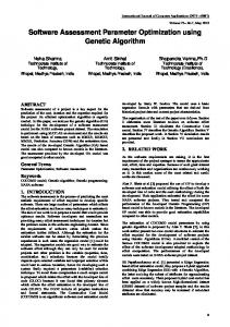
Images of the Cairo city are used to extract the required data for the training and testing purposes. First of all, having an image from the Cairo city (Urban Landsat) [19] and a corresponding image from Google map, image is labeled manually. Fig. 1 shows Cairo in Google map and the Fig. 2 is the labeled image.

Figure 2. Labeled image

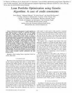
In Fig. 2 vegetation is labeled by pure green (0, 255, 0), water is labeled by pure blue and soil is labeled by pure red. There are 1665 total pixels, 555 pixels for each land cover. After labeling the image, classic NDVI was applied on the labeled pixels. Results are depicted by a histogram diagram in Fig. 3. In Fig. 3, horizontal axis is the classic NDVI value. For example, there are about 400 pixels between -0.4 and -0.2 on the horizontal axis. This histogram has three cluster centers, 0.9018 for vegetation, and 0.1161 for soil and -0.2768 for water. Intension is to derive twelve coefficients (c1 to c12) which will form (3) with maximum separation and uniform distribution. The training set contains equal number of members for each land cover type.

GA − NDVI =

c1b1 + c2 b2 + c3b3 + c4 b4 + c5 b5 + c6 b6 c7 b1 + c8b2 + c9b3 + c10 b4 + c11b5 + c12 b6

. (3)

Figure 3. The resulted histogram after applying classic NDVI on labeled image

Where, bi is the pixel value of ith band from a multispectral image. The desired histogram is the one with three centers far from each other with almost equal sample frequency for each cluster. In other words, considering 3 land covers, there can be 3 classes. On the other hand, the training set has 1665 pixels, 555 samples from each type of land cover. Therefore, goal is to find a histogram with the longest distance between their centers where each class contains 555 samples. This is an ideal condition to consider. IV.

GENETIC ALGORITHM

In order to achieve the desired histogram, an appropriate fitness function should be selected. In the reported work, the following fitness function was used:

Fitness =

Figure 1. City of Cairo in Google Map

555 − freq1 + 555 − freq 2 + 555 − freq3 hist − width

. (4)

Where “hist-width” stands for histogram width, which, is the total distance between centre locations in a histogram. The resulted histogram here has three bins, therefore, hist-width will be dist12 + dist13 + dist23. freqi is the frequency of cluster i. Aim is to minimize (4) using genetic algorithm. This function tends to be minimal when cluster centers are far from each other and each cluster contains about 555 samples.

V.

EXPRIMENTAL RESULTS

In our implementation the chromosome has twelve genes each representing one coefficient. After running GA with initial population of 80 chromosomes and after 300 generations, the following coefficients are obtained: c1…c12 = {0.423, 0.868, -1.441, -4.78, 3.77, -0.528, -0.91, 0.009, 0.241, 0.469, 0.114, -0.298} Applying these coefficients, the histogram in Fig. 4 is resulted. The resulted cluster centers in Fig. 4 are -11.8191 for soil, 5.5259 for vegetation and -3.1466 for water. Thus a new indictor with new thresholds is introduced. In the following sections, confusion matrix for the results is calculated and compared versus the results from the classic NDVI. VI.

COMPARISON WITH CLASSIC NDVI

In order to evaluate the proposed method, some other segments of the image are labeled to have a test set. TABLE I and TABLE II represent the resulted confusion matrices. Thus, true positive rate for classic NDVI is 91.99% and GA-NDVI shows 98% for this rate. Using confusion matrix, classic and GA NDVI can be compared in some other criterions as well. TABLE III provides an overall view for a comparison.

TABLE III. Comparison between GA and Classic NDVI True Positive rate False Positive Precision Recall F-score

NDVI 91.99% 0.0353 0.91 0.90 0.90

GA-NDVI 98% 0.0090 0.97 0.97 0.97

VII. INCREMENTAL REMOVAL OF THE COEFFICIENTS Using large number of coefficients in the process of land cover classification, especially, in huge sized images, will reduce the performance. Therefore, in addition to the classification precision, its performance is an important issue as well. In this section coefficients are removed one after another in ascending order and in each step F-score is calculated. The goal is to give the user a chance to decide what trade-off between accuracy and speed he/she needs. In order to do that, coefficients are initially sorted based on their absolute values. Once the coefficients are sorted, one can start with removing coefficients in an order determined in TABLE IV. Order of appearance in the sorted coefficients list represents the importance of that coefficient. Therefore, as presented in TABLE IV, coefficient c4 is the most significant coefficient and c8 is the least significant coefficient. The process starts by removing c8, then c8 and c11, etc. TABLE V presents these steps. The F-measure is a trade-off between precision and recall by combining them into a single formula. The traditional Fmeasure is the harmonic mean of precision and recall, i.e. 2PR/(P+R) where P is precision and R is recall [20].

Figure 4. Histogram obtained from GA-NDVI

The result shows two breaking points in F-measure value. The following plot shows these points. Fig. 5 shows major decrease at two points, i.e. 6 and 9. Fig. 5 shows that removing these coefficients until the coefficient at step 6 will not significantly affect the accuracy of the result. However, Fmeasure will fall down to 0.5, once the coefficient 6 is removed. Removing seventh and eighth coefficients doesn’t affect the accuracy. The ninth deletion (c7) will cause a sudden 50% decrease in accuracy (TABLE IV).

TABLE I. Classic NDVI Confusion Matrix Classified soil True soil True vegetation True water

2969 34 981

Classified vegetation 2 6533 54

TABLE IV. Coefficients in ascending order Classified water 0 0 2792

TABLE II. A NDVI Confusion Matrix

True soil True vegetation True water

Classified soil 2954 2 197

Classified vegetation 16 6560 33

Classified water 1 5 3597

Step 1 2 3 4 5 6 7 8 9 10 11 12

Removed coefficient index(i) 8 11 9 12 1 10 6 2 7 3 5 4

|Ci| 0.0096 0.1141 0.2419 0.2984 0.4238 0.4693 0.5288 0.8680 0.9101 1.4417 3.7730 4.7804

TABLE V. Removing Coefficients in Incremental Order Step

Removed coefficients

Precision

Recall

F-measure

Step

Removed coefficients

Precision

Recall

F-measure

1 2 3 4 5 6

8 8,11 8,11,9 8,11,9,12 8,11,9,12,1 8,11,9,12,1,10

0.9756 0.9780 0.9760 0.9795 0.9569 0.4340

0.9772 0.9810 0.9812 0.9820 0.9607 0.6438

0.9764 0.9795 0.9786 0.9807 0.9588 0.5185

7 8 9 10 11

8,11,9,12,1,10,6 8,11,9,12,1,10,6,2 8,11,9,12,1,10,6,2,7 8,11,9,12,1,10,6,2,7,3 8,11,9,12,1,10,6,2,7,3,5

0.3891 0.4310 0.0741 0.0741 0.0741

0.6027 0.6181 0.3333 0.3333 0.3333

0.4729 0.5079 0.1212 0.1212 0.1212

After removing five coefficients, the resulting formula is as follows: GA − NDVI =

0.8b2 − 1.4b3 − 4.7b4 + 3.7b5 − 0.5b6 −0.9b1 − 0.4b4

. (5)

For further simplification, coefficients are rounded and then compared against classic NDVI. Results are reported in TABLE VI. The proposed formula is as follows: GA − NDVI =

b2 − 1.5b3 − 5b4 + 4b5 − 0.5b6 −b1 − 0.5b4

.

(6)

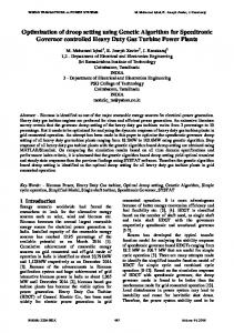
This formula keeps the classification accurate and fast. At the same time, it separates the cluster centers far from each other. Using this formula as a classifier needs new threshold values. This is because it generates different values from the previous formula (Equation 2 with 12 coefficients). These thresholds can be obtained by considering separate training samples for water, soil, vegetation and their NDVI value intervals. These thresholds can also be found considering histograms separately. The resulted intervals are [3.2398 7.2692] for vegetation, [0.9 552 1.7989] for soil and [-1.4091 0.9552] for water. Fig. 6 shows the result of GA-NDVI applied on a segment of the image of Cairo city. In the resulted image, blue pixels represent water, red pixels represent soil and green pixels represent vegetation. TABLE VI. Rounded GA-NDVI VS. Classic-NDVI Precision Recall F-measure

Rounded GA-NDVI 0.9670 0.9709 0.9690

Classic NDVI 0.9122 0.9079 0.9101

Figure 6. (top) true classified image, (bottom) The result of applying GANDVI on top (Blue is water, red is soil and green is vegetation)

VIII. CONCLUSION A new index for NDVI was introduced in this paper. The reported work starts with labelling images manually. Later on, the goal is to find twelve coefficients, so that, a linear combination of six bands of Urban Landsat image can be made. This combination can be found by applying genetic algorithm and then removing coefficients incrementally one by one until a major loss of information occurs. Smoothing the coefficients, new thresholds for land cover classification are calculated. This new index has a better separation of the classes and shows more accurate result in comparison with the classic NDVI. This index can be used to design tools e.g. MultiSpec [21] and is believed to make enhancement on a widely used index which has been applied on variety of application [22, 23]. IX.

Figure 5. F-measure trend in removing coefficients in incremental order

FUTURE WORKS

Using more general evaluation techniques with more landscape images and more sampled data, robustness of the

proposed method can be improved. This paper used Urban Landsat images as training samples that means that the formula is valid only on this satellite. For more generalization, one may create a framework in which different satellites will be supported. The proposed work can be extended to find new indicators for clouds which are widely used in weather forecasting. REFERENCES [1]

P. M. Mather, “Computer processing of remotely-sensed images,” third edition, John Wiley & Sons, Ltd June 25, 2004. [2] É. Arsenault, and F. Bonn, "Evaluation of soil erosion protective cover by crop residues using vegetation indices and spectral mixture analysis of multispectral and hyperspectral data," CATENA, vol. 62, pp. 157172, 2005. [3] X. Zhou, H. Guan, H. Xie, and J. L. Wilson, “Analysis and optimization of NDVI definitions and areal fraction models in remote sensing of vegetation,” International Journal of Remote Sensing, vol. 10, pp. 721 -751, 2009. [4] C. Hély, P. Braconnot, J. Watrin, and W. Zheng, "Climate and vegetation: Simulating the African humid period," Comptes Rendus Geosciences, vol. 341, pp. 671-688, 2009. [5] P. Lopez, P. Sirguey, Y. Arnaud, B. Pouyaud, and P Chevallier, “Snow cover monitoring in the Northern Patagonia Icefield using MODIS satellite images (2000-2006),” Global and Planetary Change, vol. 61, pp. 103-116, 2008. [6] A. M. de Asis, and K. Omasa, "Estimation of vegetation parameter for modeling soil erosion using linear Spectral Mixture Analysis of Landsat ETM data," ISPRS Journal of Photo-grammetry and Remote Sensing, vol. 62, pp. 309-324, 2007. [7] S. M. Vicente-Serrano, and J. M. Cuadrat-Prats, "Aridity influence on vegetation patterns in the middle Ebro Valley (Spain): Evaluation by means of AVHRR images and climate interpolation techniques," Journal of Arid Environments, vol. 66, pp. 353-375, 2006. [8] A. De Santis, and E. Chuvieco, “A modified version of the Composite Burn Index for the initial assessment of the short-term burn severity from remotely sensed data,” Remote Sensing of Environment, vol. 113, pp. 554-562, 2009. [9] Y. Inoue, J. Penuelas, A. Miyata, and M. Mano, “Normalized difference spectral indices for estimating photosynthetic efficiency and capacity at a canopy scale derived from hyperspectral and CO2 flux measurements in rice,” Remote Sensing of Environment, vol. 112, pp. 156-72, 2008. [10] A. Huete, K. Didan, T. Miura, E. P. Rodriguez, X. Gao, and L. G.

[11] [12]

[13] [14]

[15] [16]

[17] [18]

[19] [20] [21] [22]

[23]

Ferreira, "Overview of the radiometric and biophysical performance of the MODIS vegetation indices," Remote Sensing of Environment, vol. 83, pp. 195-213, 2002. Z. Jiang, A. R. Huete, and K. Didan, "Development of a two-band enhanced vegetation index without a blue band," Remote Sensing of Environment, vol. 112, pp. 3833-3845, 2008. Z. Jiang, A. R. Huete, J. Chen, Y. Chen, J. Li, and G. Yan, “Analysis of NDVI and scaled difference vegetation index retrievals of vegetation fraction,” Remote Sensing of Environment, vol. 101, pp. 366-378, 2006. S. R. Freitas, and M. C. S. Mello, "Relationships between forest structure and vegetation indices in Atlantic Rainforest," Forest Ecology and Management, vol. 218, pp. 353-362, 2005. X. Yao, Y. Zhu, Y. Tian, and W. Feng, “Exploring hyperspectral bands and estimation indices for leaf nitrogen accumulation in wheat,” International Journal of Applied Earth Observation and Geoinformation, vol. 12, pp. 89-100, 2010. F. Belda, and J. Meliá, "Relationships between climatic parameters and forest vegetation: application to burned area in Alicante (Spain)," Forest Ecology and Management, vol. 135, pp. 195-204, 2000. Y. Julien, and J. A. Sobrino, “The Yearly Land Cover Dynamics (YLCD) method: An analysis of global vegetation from NDVI and LST parameters,” Remote Sensing of Environment, vol. 113, pp. 329-334, 2009. B. Martinez, and M. A. Gilabert, “Vegetation dynamics from NDVI time series analysis using the wavelet transform,” Remote Sensing of Environment, vol. 113, pp. 1823-1842, 2009. J. Epting, D. Verbyla, and B Sorbel, “Evaluation of remotely sensed indices for assessing burn severity in interior Alaska using Landsat TM and ETM+,” Remote Sensing of Environment, vol. 96, pp. 328-339, 2005. Urban Landsat images: http://sedac.ciesin.org/ulandsat/data.jsp as visited on 2009. C. D. Manning, “An introduction to information retrieval”, Cambridge University Press, 2008. L. Ryan, University of New Hampshire, “Creating a Normalized Difference Vegetation Index (NDVI) image Using MultiSpec", The GLOBE Program, page 2, 1997. A. R., Huete, K. Didan, Y. E. Shimabukuro, P. Ratana, S. R. Saleska, L. R. Hutyra, W. Yang, R. R. Nemani, and R. Myneni , “Amazon rainforests green-up with sunlight in dry season,” Geophysical Research Letters, vol. 33, 2006. C. C. Funk, and M. E. Brown, “Intra-seasonal NDVI change projections in semi-arid Africa,” Remote Sensing of Environment, vol. 101, pp. 249-256, 2006.