Volume Subdivision based Hexahedral Finite Element Meshing of domains with interior 2-manifold boundaries Chandrajit L. Bajaj∗ Department of Computer Science and The Institute for Computational Engineering and Sciences Lalit C. Karlapalem† Department of Mechanical Engineering and The Institute for Computational Engineering and Sciences The University of Texas at Austin
Abstract
Besides Engineering and physics applications, meshes are also utilized in physically based animations, computer graphics [Schneiders et al. 1996], [Kent et al. 1992]. The additional requirements of hexahedral meshing make it more demanding [Pascal and George 2000].
We present a subdivision based algorithm for multi-resolution Hexahedral meshing. The input is a bounding rectilinear domain with a set of embedded 2-manifold boundaries of arbitrary genus and topology. The algorithm first constructs a simplified Voronoi structure to partition the object into individual components that can be then meshed separately. We create a coarse hexahedral mesh for each Voronoi cell giving us an initial hexahedral scaffold. Recursive hexahedral subdivision of this hexahedral scaffold yields adaptive meshes. Splitting and Smoothing the boundary cells makes the mesh conform to the input 2-manifolds. Our choice of smoothing rules makes the resulting boundary surface of the hexahedral mesh as C2 continuous in the limit (C1 at extra-ordinary points), while also keeping a definite bound on the condition number of the Jacobian of the hexahedral mesh elements. By modifying the crease smoothing rules, we can also guarantee that the sharp features in the data are captured. Subdivision guarantees that we achieve a very good approximation for a given tolerance, with optimal mesh elements for each Level of Detail (LoD).
In this paper, we present a volumetric subdivision based algorithm for Hexahedral mesh generation. We can deal with boundaries having multiple connected components and of arbitrary genus, while guaranteeing that the resulting boundary conforming volumetric mesh is sensitive to surface features.
CR Categories: I.3.5 [Computer Graphics]: Computational Geometry and Object Modeling—Curve, surface, solid, and object representations; J.2 [Computer Applications]: Physical Sciences and Engineering—Engineering Keywords: mesh generation, hexahedral meshing, 3D meshing, subdivision meshes
1
Introduction
1.1
Figure 1: The input 2-manifold boundary of the knee dataset comprising of the Femur, Patella and Tibia bones (3 objects) is shown in (a). A simplified inter-object Voronoi subdivision is shown in (b). The mesh shown in (c) is the volume exterior to the 2-manifold boundaries and bounded by the domain. (d) shows the boundary surface of the hexahedral mesh, and (e), (f) and (g) show cross sections of the domain, interior and exterior hexahedral meshes.
Motivation
Finite Element Meshes have found various applications in diverse fields like design, modeling, CFD and solutions to differential equations in areas like microelectronics, Aerodynamics and Engineering. In the volume case, FE Meshes mostly have tetrahedral or hexahedral elements. Hexahedral elements have wider applications because they offer more degrees of freedom per node compared to their tetrahedral counterparts. Due to this, fewer mesh elements are required in general to form a finite element mesh.
1.2
Given a bounding rectilinear domain containing embedded 2manifold boundaries of arbitrary genus and topology, construct a structured hexahedral mesh of the domain conforming to the 2manifold boundaries.
∗ e-mail:
[email protected] † e-mail:
Hexahedral Meshing Problem
[email protected]
Copyright © 2006 by the Association for Computing Machinery, Inc. Permission to make digital or hard copies of part or all of this work for personal or classroom use is granted without fee provided that copies are not made or distributed for commercial advantage and that copies bear this notice and the full citation on the first page. Copyrights for components of this work owned by others than ACM must be honored. Abstracting with credit is permitted. To copy otherwise, to republish, to post on servers, or to redistribute to lists, requires prior specific permission and/or a fee. Request permissions from Permissions Dept, ACM Inc., fax +1 (212) 869-0481 or e-mail
[email protected]. AFRIGRAPH 2006, Cape Town, South Africa, 25–27 January 2006. © 2006 ACM 1-59593-288-7/06/0001 $5.00
The input 2-manifold boundaries can be listed either as a level set of known topology or it could be explicitly mentioned as a face indexed collection. We also define an object to be a simply connected 2-manifold enclosing finite volume. Thus, the input 2-manifold boundaries can be treated as a set of objects. This is shown in
127
Figure 1. The domain consisting of three objects and their final hexahedral meshes are shown.
2.1
Hexahedral meshing is still a relatively undeveloped research area. Much more research has been published for tetrahedral meshing [Pascal and George 2000], [Owen 1998].
The first step in our Hexahedral Meshing (henceforth HexaMeshing) algorithm is to partition the domain and isolate each object. This can be achieved by using medial surfaces [Price et al. 1995], [Price et al. 1997] as inter-object separators which can be approximated by Voronoi diagrams [Sheffer et al. 1998]. Typically, if the domain contains multiple connected components, then Voronoi diagrams have been in the past used [Bajaj 2005]. Each of these subregions is then meshed individually as follows: An initial hexahedral scaffold is created that provides a rough approximation to the 2-manifold boundaries. It is then recursively refined using subdivision methods to get a conforming fit with respect to the given 2-manifold boundaries. Here, we present the details of our HexaMeshing algorithm.
1.3
Mitchell [1996] has given theoretical proof that any connected 3D domain with an even number quadrilateral boundary faces can be partitioned into a hexahedral mesh that conforms to the boundary. Eppstein [1996] shows that any polyhedron forming a topological ball with even number ‘n’ of quadrilateral boundary faces can be partitioned into O(n) topological cubes. Numerous approaches have been proposed and investigated for hexahedral meshing. The two most popular strategies for automatic hexahedral mesh generation are (1) First meshing the boundary of the mesh and then advancing the meshed surface into the volume and (2) Meshing the volume based on regular grids and intersecting the grid with the boundary. While, in general, the first approach faces the problem of properly closing the advancing fronts when they meet in the interior, the second is problematic with respect to mesh quality and proper feature resolution at the boundary.
Input and Output Format
We represent a hexahedron as a collection of 8 vertices. The topological information about its faces and edges can be found out by traversing the vertex list in an ordered fashion. e.g. The “Front” face of the hexahedron is given by vertices 1-2-3-4, while the “Far” face is given by 5-6-7-8, and so on. All points on a face are strictly co-planar within a tolerance. To achieve numerical robustness as in [Fortune 1996], we define a tolerance and perform all floating point operations using this tolerance. The input 2-manifold boundaries are specified as a boundary representation of triangles.
1.4
Perhaps the most common method of generating hexahedral meshes is by using Voronoi diagrams [Owen 1998]. The given domain is first split into sub-volumes by using the Voronoi diagram. Each of the sub regions are then meshed using other standard techniques like sweep [Lai et al. 1996], mapping [White et al. 1995] or midpoint subdivision [Sheffer et al. 1998], [Li et al. 1995]. The medial axis of an object is closely related to the Voronoi diagrams. It is in fact a subset of the boundaries of the Voronoi regions, if the geometric objects are B-rep elements. Techniques based on medial surface subdivision [Price et al. 1995], [Price et al. 1997] have also been experimented with. In this, the medial axis of the object is constructed and meshed using quad and triangular elements. These are extruded to the boundary at both sides of the medial surface. Mixed cell type elements (tetrahedra, pyramids, hexahedra) can be present, which are split into hexahedral elements. A variant of the Voronoi diagram called the Space Twist Continuum (STC) [Tautges et al. 1996] has also been successfully used in the meshing software CUBIT [White et al. 1995]. STC is a way of representing the dual of the hexahedral mesh as a simple non-degenerate arrangement of surfaces. It is built in an incremental fashion using Advancing Front Techniques (AFT) like the Whisker Weaving algorithm [Tautges et al. 1996]. Plastering methods have also been used, where the boundaries are first meshed and then extruded inside the solid [Canann 1991]. Sweeping methods [Lai et al. 1996] and Mapping techniques [White et al. 1995] have also been successfully used for generating Hexahedral meshes.
Contributions
In this paper, we present a robust and automatic algorithm for creating hexahedral meshes conforming to arbitrary geometries, with guaranteed mesh quality. The algorithm that we present has several advantages over the conventional approaches: (1) We extend the subdivision scheme to the case of a bounding cuboid with embedded arbitrary 2-manifold boundaries. (2) Recursive subdivision allows for easy creation of an hierarchial index structure and also yields adaptive control over the size of the hexahedral elements. (3) Conforming to the given geometry requires a careful tradeoff between mesh quality, number of mesh elements and accuracy of the mesh. Using intuitive parameters, we strike a balance between these. (4) The algorithm is well defined and valid for arbitrary and complex geometries. (5) Multi-resolution guarantees that we achieve a very good approximation for a given tolerance and also provides a limit on the number of elements for each level. (6) Feature identification along with the crease smoothing rules ensure that the sharp features are preserved in our final mesh. Finally, the algorithm is robust and simple, yet elegant to implement.
Alternatively, research has also been done on some grid-based methods. The given object is embedded into a regular hierarchical Octree grid. Either higher order elements can be used to represent the exact boundary of the surface by intersecting it with the grid, or body-fitting techniques can be used to represent these boundary elements [Schneiders et al. 1996]. Dual contouring has also been used by Zhang et al [2005] for extracting hexahedral meshes from imaging data. They first convert the imaging data into volumetric representations using distance fields, and then use dual contouring to extract the surface mesh [Zhang and Bajaj 2005]. Also, from a look-up table based on the function values of each cell, they can extract the conforming volumetric mesh for the domain. Using dual contouring over primal contouring guarantees that the resulting mesh has optimal elements and can preserve sharp features [Zhang and Bajaj 2005].
In section 2, we present an outline of the relevant prior work. Our HexaMeshing algorithm is described in Section 3. In section 4, we present the results of our algorithm. In section 5, we conclude by outlining some areas of future work.
2
Hexahedral Meshing
Previous work
The three closely related fields of meshing related to our problem are described in this section.
Finally, since, tetrahedral meshing is a much advanced field, a tetrahedral mesh of the given geometry can be generated first. Each
128
Approximating in which the vertices of the coarser tiling are used to compute the vertices of the refined tiling or
tetrahedron is then split into 4 hexahedra by introducing Steiner points at the centroid and at each of the edges and faces [Eppstein 1996]. However, the number of hexahedral elements is too large and often justifies the exploration for other direct hexahedral meshing algorithms.
Interpolating where the original control points defining the surface are also points of the limit surface, which allows controlling it in a more intuitive manner.
Sabin has proposed a few criteria for comparing the different schemes for hexahedral mesh generation [1991]. Mesh locality, boundary surface continuity and orientation independence are some important factors while evaluating different schemes, along with adaptivity of the mesh and control over element shape [Sabin 1991].
2.2
Traditional schemes like Catmull-Clark subdivision schemes [Catmull and Clark 1978] work for surfaces of arbitrary topology. Different averaging masks are provided for edge, face and boundary vertices. Also, the masks differ for odd (vertices inserted at the current level) and even (vertices inherited from the previous level) vertices. Loop’s subdivision scheme [1987] is based on a three directional box spline and works for triangular meshes. It constructs a C2 surface in the limit (C1 at the extra-ordinary vertices of lesser valency). The averaging masks are different for odd-even and interiorboundary vertices. However, the averaging masks for most of these algorithms are not intuitive.
Quality of Meshes
Meshes could be categorized depending on the element shapes (tetrahedral or hexahedral) or mesh topology (structured or unstructured). Here, we focus on the following aspects of Mesh quality.
Bajaj et al [2002] introduced a new subdivision scheme called as Multi Linear Centroid Averaging (MLCA). This subdivision scheme is in any number of dimensions. At each level, they first split the volume using multi-linear splitting and then the vertices are smoothed using a simple averaging rule. The main contribution of this paper is in separating the vertex insertion step from the vertex re-positioning step. Also, they have an uniform vertex averaging mask which takes care of both the interior and the boundary vertices(“crease smoothing”). In the bi-variate (surface) case, this can be thought of simply as re-positioning the vertex at the centroid of the centroids of the four quadrilaterals that share the vertex. Subdivision based schemes have also been recently used in hexahedral meshing of particles for meshing a disjoint collection of spheres of different radii [Bajaj 2005].
Optimal meshing: It can be shown that the running time of the finite element method is O(na ), where ‘a’ is at least 1 depending on the solver used for solving the sparse linear equations [Mitchell and Vavasis 2000], [Bern et al. 1990]. A theoretical proof for the optimal number of tetrahedral elements in the mesh is given by Mitchell et al in [2000]. Error Bounds: In meshing with linear elements, we are approximating the true function with piecewise linear functions. Thus the accuracy of the estimation is also an important factor that can affect other parameters like Stiffness matrices [Berzins 1998]. Shewchuk [2002] gives a good estimate on the error bounds for linear meshing elements. Feature Sensitive Meshing: Features are defined by the surface topology of the input domain. While this is inherent in algorithms based on Voronoi regions as they consider the local neighborhood of the surface, for grid-based methods, this is an important issue. Extensive use of Body-fitting techniques have been made [Schneiders et al. 1996] to make the mesh conform to the given geometry. Higher order elements have also been used to represent the surface at the boundary cells.
2.3
3
HexaMeshing Algorithm
The sketch of our algorithm is as follows: 1. We use Voronoi Diagrams to create inter-object partitioning of the given domain. 2. Each Voronoi cell is then decomposed into hexahedral elements using a radial subdivision scheme.
Subdivision
3. Recursive subdivision of the initial hexahedral scaffolding gives a C2 smooth boundary surface of the final hexahedral mesh (C1 at extra-ordinary vertices).
Subdivision defines a smooth curve or surface as the limit of a sequence of successive refinements. For this, additional vertices are introduced into the original geometry. To determine where to place the new points on the given geometry, we need to look at some of the properties like [Schroder et al. 1999] 1 :
3.1
Efficiency: The location of new points should be computed with a small number of floating point operations.
Voronoi Subdivision and Simplification
If the input 2-manifold boundaries contain more than one object, we separate each object into its own convex region that can then be meshed separately. For this, we use Voronoi diagrams. We ensure that the sampling of the 2-manifold boundaries is sufficient enough to construct a topologically accurate Voronoi Diagram and its dual the Delaunay Triangulation [Cheng et al. 2004], [Boissonnat and Oudot 2003]. In case the criterion is not met, we follow the set of guidelines mentioned in Cheng et al in [2004] for their “Topology Sampling” step.
Local Definition: The rules used to determine the position of the new points should depend closely on their immediate neighbors. Simplicity: Determining the rules themselves should be a simple process with a small number of rules. Continuity: Resulting boundary curves and surfaces need to be differentiable so that properties like continuity and gradients can be readily obtained.
Next, we construct the Voronoi Diagram for the domain comprising of the complete set of vertices of the input 2-manifold boundaries. Dey et al [2004] have shown that the Voronoi Diagram of the sampling of the 2-manifold boundaries can also be used to extract the Medial Surface of the domain. We use this structure to partition the domain into (convex) Voronoi cells, such that each cell contains
Depending upon the particular application, some of these properties might be important in the choice of a subdivision scheme. Broadly, these schemes can be categorized as 1 [Schroder
et al. 1999] provides an excellent review of the various Subdivision techniques.
129
We notice that the dual of the Voronoi Diagram is the Delaunay Triangulation of the domain. From this, we can extract a set of critical points in each Voronoi cell [Dey et al. 2003]. These critical points are defined as the local maxima or saddle points of the global distance function. Dey et al [2003] use these critical points to construct a set of stable manifolds locally, for their segmentation routine. In our case, we use the same set of critical points to provide us with a good decomposition of the Voronoi cell into simplified sub-regions, with each sub-region enclosing a finite volumetric portion of the input 2-manifold boundaries. Next, we split each of these sub-regions into hexahedra using the radial subdivision scheme outlined in [Bajaj 2005]. However, we have to guarantee that the partitioning is topology conserving and does not produce any self-intersections. For this, we check whether radial lines from these interior points to the boundary faces of the Voronoi cells result in multiple intersections with the enclosed 2-manifold boundary enclosed within each sub-region. In other words, we need to determine if the 2-manifold boundary enclosed within each sub-region is topologically equivalent to a star shape [Kent et al. 1992] or not. If the enclosed 2-manifold boundary intersects all the radial faces of the sub-region, then it leads to a valid radial hexahedral partitioning of the sub-region. In case this condition is not true, then we split the sub-region laterally using the medial surface, till this criterion is satisfied. Also, note that the radial partitioning of these sub-regions creates an initial scaffolding that is a conforming hexahedral mesh, in that there are no hanging nodes.
Figure 2: Voronoi Region: The figure to the left shows the Voronoi regions for the four ellipsoids. The mesh to the right shows the Voronoi Diagram of the domain. only one object and a collection of convex Voronoi cells define an object. We perform a Voronoi simplification by topology controlled decimation to reduce the number of Voronoi cells [Dey and Zhao 2004]. This is shown in Figure 2 where the input is a set of ellipsoids. The Voronoi Diagram of the domain and the initial hexahedral scaffolding is shown.
3.3
We maintain an Octree data-structure [Glassner 1984] to minimize the number of computations. During the tri-linear splitting of a cell, we need to maintain topological information about the 2-manifold boundary that is contained within each cell. This data is also useful while classifying the vertices of the hexahedron. These calculations are done every time a cell is split and a new vertex is introduced. Thus, to reduce the number of ray-triangle intersections, we use the Octree data-structure.
Figure 3: The first picture is the input human ’femur knee’ dataset. The center picture shows the Gouraud shaded hexahedral mesh after 7 levels of cell splitting and 10 rounds of smoothing. The last picture is a zoom-in of the region showing the multiple connected components of the final hexahedral mesh.
3.2
Hexahedral Recursive Subdivision and Quality Enhancement
For this, we use standard Octree generation algorithms. To traverse the Octree from a given point along a given direction, we discretize the ray and find the first point on the ray which is outside the given cell. As we have a regular grid, finding the grid cell that contains this point is a trivial computation. Note that the Octree depth should be more than or equal to the levels of subdivision of the mesh.
Hexahedral Scaffolding of Volumes
Tolerance: Every time we introduce new vertices into the mesh, we need to classify these vertices. For this, we compare the Euclidean distance of the vertex to the 2-manifold boundary, with the user specified tolerance. We round off the tolerance to the nearest power of 2 and the exponent determines the level of subdivisions in our algorithm. Note that this parameter along with the Octree resolution define the optimal number of elements in the mesh for that resolution.
The Medial Surface computed above also provides us with a skeletonization of the domain, which we use to construct an initial hexahedral scaffolding for each object. Once we construct the Voronoi Diagram for the complete domain, we then look at each Voronoi cell to determine the topology of the enclosed object within each cell as well as a preliminary hexahedral decomposition (scaffolding). Bajaj has shown [2005] how to construct a hexahedral scaffolding of arbitrary radius spheres. This could be extended to convex and star shaped objects [Kent et al. 1992] by selecting a center point from which lines in radial directions intersect the surface boundary in singly.
Cell Splitting During each level of subdivision, we split the current mesh adaptively. For adaptive splitting, each hexahedron containing a part of the 2-manifold boundary, is split into 8 subcells using the tri-linear splitting scheme [Bajaj et al. 2002]. For uniform splitting, all the hexahedra in the mesh are split. While uniform splitting generates more hexahedral elements,
The centers are joined with the boundaries and the centroids of these boundary faces to form quad based pyramids, which can be used to construct hexahedra. Details of this scheme are presented in [Bajaj 2005]. Our goal here is to identify such interior points within each Voronoi cell for non-convex objects.
130
it guarantees no hanging points (T-junctions). On the other hand, adaptive splitting introduces hanging points into the mesh (see figures 11, 8). After splitting the mesh till the final resolution, we smooth the vertices. The number of smoothing steps is also an user-defined parameter for our algorithm.
The adaptive cell splitting criteria is shown in Figure 5. In certain applications, it is not permissible to have hanging nodes in the meshes. We can adopt a technique similar to the one used by Schneiders [1996] and Zhang et al [2005] where they provide templates to extract adaptive hexahedral meshes. Using this approach, we can strike a good balance between feature adaptivity and optimality of mesh elements. Feature Detection Repeated application of centroid smoothing (described below) can smooth out the sharp features. In certain cases, these are important and need to be preserved. Hence, just before creating the mesh at the final resolution, we perform a feature detection test. We use a feature detection algorithm, similar to the one used by Kobbelt et al in [2001]. The enhanced distance field is computed for all the boundary cells. The exact points and their surface normals on the resulting iso-surface are then sampled. Performing the two simple angle checks outlined in [Kobbelt et al. 2001], determines if the cell has any embedded features. The boundary vertices of the feature cells are tagged. The crease smoothing rules are applied for these boundary vertices, while the cell averaging rules are used for all the boundary vertices.
Figure 4: The topologically different cases for the boundary cells of each Voronoi cell. Here, we show their corresponding quadralizations.
Centroid Smoothing After creating the mesh at the lowest resolution, we smooth the boundary vertices using the MLCS algorithm by Bajaj [2005] to conform to the input 2-manifold boundary.
Tri-linear splitting of a hexahedron introduces new vertices into the mesh. These need to be classified as inside-outside and interior-boundary with respect to the input 2-manifold boundary. For this, we compute the distance of the vertex to the 2-manifold boundary using the signed distance calculation given by Payne et al in [1992]. This gives us the complete classification of the vertex. After classifying the vertices, we follow the same classification scheme for the hexahedral cells also. The different topological arrangements of the boundary cells which approximate the smooth surfaces or surfaces with creases, along with their corresponding tessellations are shown in Figure 4. The extended table of cases based on critical point analogs of tri-linear functions given in [Lopes and Brodlie 2003] could also be used, if one needed to accurately disambiguate the correct topology. However, these cases of multiple saddle points within a cell rarely occur in practice. Cases like 4.1.2, 6.1.2, 7.4.1, 10.1.2, 13.3, 13.4, 13.5.1 and 13.5.2 are topologically equivalent to a “tunnel” and are difficult to mesh, while the cells with the other cases can be recursively subdivided till they fall into the basic cases shown in Figure 4.
In the bi-variate case, for each vertex, we compute the centroids of the boundary quads that share the vertex. The vertex is re-positioned to the centroid of these centroids. In the tri-variate case, the interior (and exterior) hexahedra are smoothed using the vertex smoothing rule given by Bajaj et al in [2002]. The crease smoothing rules are used in repositioning the boundary vertices of the mesh which are close to the identified “features” in the 2-manifold boundaries. The interior vertices are left unchanged during this step. If x ∈ ℜ3 and xi ∈ ℜ3 for i = 1, ..., m are its neighboring vertices, then an edge vector is defined as ei = xi − x with i = 1, ..., m and the Jacobian J = [e1 , ..., em ] [Zhang and Bajaj 2005] (for hexahedral meshes, m=3). The determinant of the Jacobian matrix is called as the Jacobian or scaled Jacobian, if the edge vectors are normalized. An element is inverted if one of its J ≤ 0. The condition number of the Jacobian is de|J| . Our goal is to fined as κ (J) = |J||J −1 |, where |J −1 | = det(J) remove the inverted elements and improve the worst condition number. Thus, after each smoothing iteration, we check the positiveness of the Jacobian of the hexahedral elements and this provides a bound on the number of smoothing steps that we can perform.
If after a cell is split, all the 8 vertices are classified as boundary, then it will lead to a hexahedral cell element with all 6 faces as boundary. Hence, we do not perform the split in such cases. Note that the actual positioning of the new vertices is determined by the tri-linear splitting rules by Bajaj et al in [Bajaj et al. 2002], while the actual topology of the new hexahedra is determined from the lookup table shown in Figure 4.
Mesh Decimation After smoothing, we merge some of the cells to control the
131
number of elements in the mesh. This can be done in the following two ways:
creases, the finer details in the mesh are also captured. The pictures at the bottom row show the cross sectional cuts of the mesh in the Co-ordinate planes. The adaptive cell splitting scheme guarantees that larger cells are present in the interior (and exterior) of the mesh.
(a) Merge the interior cells: By performing an adaptive splitting of cells, we maintain feature sensitivity in our mesh. The interior (and exterior) of the mesh has larger elements compared with the boundary, where we split the cells to get a more accurate representation.
Figure 11 shows the results for the human Femur knee dataset. Starting from the input cuboid, it is first recursively subdivided till a certain resolution is reached. This is shown in the images in the top row. Note that at this stage, no smoothing has been performed on the mesh. The first two images in the bottom row show the results before and after 5 levels of smoothing. The final meshes show the cross sectional views.
(b) Merge the boundary elements: This is a crucial step in the mesh decimation process. We merge the cells that are flat over the boundary surface of the mesh. Closer inspection reveals that we can merge only the cells that have exactly one boundary face each and share an interior face. For this, we have a parameter merging tolerance. We compare the surface normals of the boundary faces of the candidate cells and if they are within this tolerance, we merge the cells. Note that if the tolerance is loose, then vacant regions are introduced into the mesh, while tight tolerances do not perform good decimation.
Figure 7 shows the effect of successive levels of smoothing on the head dataset. Each boundary vertex is moved to the centroid of the centroid of the boundary faces sharing it.
Cell merging introduces hanging points into the mesh and is left to be treated by the solver [Schneiders et al. 1996]. Note that this is an optional step. We could remove all hanging points from our mesh by simply performing uniform splitting of the cells and not merging the boundary elements. Please see Figure 5.
Figure 5: The Fandisk dataset. (a) shows mesh after 8 levels of splitting and 10 levels of smoothing. A cross sectional view (b) shows the adaptive splitting criteria. Note that uniform splitting would provide a mesh without any hanging nodes as shown in (c).
4
Results
Here, we present the results of our Hex meshing algorithm in detail. We also present some potential application domains, where this scheme, can be used with some modifications. Figure 6 shows the results on the mannequin “human head” dataset for increasing Levels of Detail. The pictures from left to right show the results of the smoothing algorithm. It can be seen that progressive smoothing steps makes the mesh conform to the input 2-manifold boundary and also yields a surface that is C2 continuous in the limit and C1 at extraordinary points. The theoretical proof of the continuity is given in [Bajaj et al. 2002]. The results of the adaptive splitting are shown in the next two rows. As the resolution in-
Figure 6: The mannequin head model. The Level of Detail increases from top to bottom for levels 4, 5 and 6. The first column shows the initial mesh before smoothing. The second column shows the mesh after 5 steps of smoothing and the next column after 10 steps. The bottom row shows the cross-sections along the three Co-ordinate planes. All meshes have been Gouraud shaded. For clarity, we do not show the wireframe of the meshes in the second last row. No surface decimation has been performed on the meshes.
132
The ability of our algorithm to preserve features is shown in Figures 6 and 10. Notice that for the mechanical part dataset, we performed only 5 steps of smoothing, while for all other datasets, we perform 10 steps. Repeated smoothing on the sharp edges tends to introduce a “filleting” effect on the edge as shown in the enlarged views. Hence, fewer number of smoothing steps are chosen for such datasets. Figure 8 shows the mesh that is exterior to the 2-manifold, but bounded by the cuboid.
part of the 2-manifold boundary. Also, during the split operation additional vertices are introduced into the mesh. We need to ensure that these are not repeated. Hence, we also need to go through the vertex list once for each new vertex. We do this in constant time by using a Hash-table for the mesh vertices. Thus, the Cell splitting operation takes O(8d ) time, where d is the levels of subdivision that we achieve. (4) Boundary Smoothing: Each boundary vertex is to be repositioned depending on its neighbors. We maintain backpointers for each vertex pointing to the cells sharing it. Thus, this operation is O(n) where n is the number of boundary cells in the mesh at the final level. Thus, the total time complexity of the algorithm is dominated by the exponential 8d term for recursive subdivision of the Voronoi cells. The Normal Flipping, Voronoi Diagram and Octree creation are all done only once. Our implementation of the algorithm is in C++ using a MSVC6.0 compiler. We tested our algorithm on a PC equipped with a Pentium III 800Mhz processor with 256MB of RAM and a GEForce 3 video card. Table 1 encapsulates the performance results for the datasets shown.
Figure 7: The sequence shows the enlarged views of certain regions in the mannequin head dataset. The initial mesh after 7 levels of splitting is shown in (a). The mesh after 1 smoothing step is shown in (b). (c) is after 3 steps, (d) after 5 and (e) is after 10 steps.
5
Conclusions
We have presented a generic algorithm for constructing the hexahedral meshes from a rectilinear domain with embedded 2-manifold boundaries of arbitrary genus.
The adaptive splitting scheme is shown in figures 11 and 8 for the Fandisk dataset. Note the mesh that is exterior to the input 2-manifold boundary is dense around the 2-manifold boundary and is coarse everywhere else. Figure 9 shows a smooth 2-manifold boundary and its hierarchical hexahedral meshes. Figure 12 show the results for the 3D imaging data. First, the level sets were extracted using dual contouring and then this was used as input for our HexaMeshing algorithm. The figure shows the meshes for both the skin and skull iso-values. 4.1
Figure 8: (a)Mechanical part dataset: The mesh bounded by the cuboid and exterior to the 2-manifold boundary. A cross sectional view is shown in (b). Note the adaptive splitting criteria produces a few number of hexahedral elements.
Time Complexity
Here, we discuss the time-complexity of our algorithm and present the run-time results of a few selected datasets. Each step of our algorithm is discussed here:
Our algorithm, while suited primarily for static meshes, can also be extended to handle dynamic meshes, where the embedded 2-manifold boundaries are deformed. Each time the 2-manifold boundary is deformed, we update the list containing the boundary cells. Then, a conforming hexahedral mesh can be extracted locally for these boundary cells and their first neighbors using the subsequent recursive subdivision step.
(1) Normal Flipping and Octree creation: If the input 2manifold boundaries contain n triangles, then each triangle has to be processed d times, where d is the Octree depth. Hence, the total cost is O(dn). (2) Voronoi Diagrams: If the input 2-manifold boundaries contains n vertices, then the total cost for creating the Voronoi Diagram for the domain is O(n2 ) in the worst case and O(nlogn) in the average case [Dey and Zhao 2004].
Improving mesh properties like optimality in number of meshing elements without any hanging nodes is an area of future work. Starting from an uniform mesh, adaptive meshes can be generated [Wada 2002], with some limitations.
(3) Cell Splitting: For each cell in the mesh at a given resolution, we split it into its 8 constituent cells if it contains any
133
Datasets Head Mechpart UNC Skin UNC Skull Knee Fandisk Chesspiece
Triangles 25,532 26,624 204,340 192,668 3,798 12,946 13,312
Grid Resolution 65×65×65 65×65×65 129×129×129 129×129×129 128×128×128 129×129×129 65×65×65
Table 1: Performance results Mesh Vertices Mesh Elements 266,820 185,538 110,577 74,894 271,664 2,472,552 370,416 3,433,596 387,359 1,576,896 966,330 4,12,973 104,558 36,199
Splitting 7 7 7 7 7 8 6
Smoothing 10 5 10 10 10 10 15
Runtime (s) 183 48 754 871 887 1,524 187
B ERZINS , M. 1998. Mesh Quality: A function of Geometry, Error Estimates or both? Tech. Rep. 229238, 7th International Meshing Roundtable, Sandia National Labs, October. B OISSONNAT, J., AND O UDOT, S. 2003. Provably Good Surface Sampling and Approximation. Eurographics Symposium on Geometry Processing (SGP), 9–19. C ANANN , S. 1991. Plastering and Optismoothing: New Approaches to Automated 3D Hexahedral Mesh Generation and Mesh Smoothing. PhD thesis, Brigham Young University, Provo, UT. C ATMULL , E., AND C LARK , J. 1978. Recursively generated B-spline Surfaces on arbitrary Topological Meshes. Computer Aided Design 16(6), 350–355. C HENG , S.-W., D EY, T., R AMOS , E., AND R AY, T. 2004. Sampling and Meshing a Surface with Guaranteed Topology and Geometry. Proceedings of 20th Symposium of Computational Geometry, 180–289.
Figure 9: The first picture is the input Chesspiece dataset. The next picture shows the mesh after 6 levels of splitting followed by 10 levels of smoothing. A cross-section is also shown.
6
D EY, T., AND Z HAO , W. 2004. Approximating Medial Axis from the Voronoi Diagram with Convergence Guarantee. Algorthmica 38(1), 179–200.
Acknowledgments
The authors are grateful for the system and software help provided by Anthony Thane, Vinay Siddavanahalli, Yongjie Zhang, Sangmin Park and Jianguang Sun. This work was supported in part by NSF grants ITR-ACI-0220037, EIA0325550 and NIH-IROI-GM074258.
D EY, T., G IESEN , J., AND G OSWAMI , S. 2003. Shape Segmentation and Matching with Flow Discretization. Proccedings of Workshop on Algorithms and Data Structures, 25–36. E PPSTEIN , D. 1996. Linear Complexity Hexahedral Mesh Generation. Symposium on Computational Geometry, 58– 67.
References
F ORTUNE , S. 1996. Robustness Issues in Geometric Algorithms. Applied Computational Geometry, Springer Lecture Notes in Computer Science, 9–14.
BAJAJ , C., S CHAEFER , S., WARREN , J., AND X U , G. 2002. A Subdivision Scheme for Hexahedral Meshes. Journal of Visual Computer, special issue on subdivision 18, 409–420.
G LASSNER , S. 1984. Space Subdivision for Fast Ray Tracing. IEEE Computer Graphics and Applications 4(10), 15–22.
BAJAJ , C. 2005. A Laguerre Voronoi Based Scheme for Meshing Particle Systems. Japan Journal of Industrial and Applied Mathematics, (JJIAM) 22(2), 167–177.
K ENT, J., C ARLSON , W., AND PARENT, R. 1992. Shape Transformation for Polyhedral Objects. In In Computer Graphics (Proceedings of ACM SIGGRAPH 92), ACM, 47–54.
B ERN , M., E PPSTEIN , D., AND G ILBERT, J. 1990. Provably Good Mesh Generation. IEEE Symposium on Foundations of Computer Science, 231–241.
KOBBELT, L., B OTSCH , M., S CHWANECKE , U., AND S EI DEL , H. 2001. Feature Sensitive Surface Mesh Extraction
134
from Volume Data. In Proceedings of SIGGRAPH 2001, ACM Press / ACM SIGGRAPH, Computer Graphics Proceedings, Annual Conference Series, ACM, 57–66.
S ABIN , M. 1991. Criteria for Comparison of Automatic Mesh Generation Methods. Advances in Engineering Software 13(5), 220–25.
L AI , M., B ENZLEY, S., S JAARDEMA , G., AND TAUTGES , T. 1996. A Multiple Source and Target Sweeping Method for Generating All-Hexahedral Finite Element Meshes. 5th International Meshing Roundtable, Sandia National Laboratories, 217–228.
S CHNEIDERS , R., S CHINDLER , R., AND W EILER , F. 1996. Octree-Based Generation of Hexahedral Element Meshes. 5th International Meshing Roundtable, Sandia National Labs, 205–216. S CHNEIDERS , R. 1996. Refining Quadrilateral and Hexahedral Element Meshes. 5th International Conference on Grid Generation in Computational Field Simulations, 679–688.
L I , T. S., M C K EAG , R., AND A RMSTRONG , C. G. 1995. Hexahedral Meshing using Midpoint Subdivision and Integer Programming. Computer Methods in Applied Mechanics and Engineering 124, 171–193.
S CHRODER , P., Z ORIN , D., D E ROSE , T., KOBBELT, L., S TAM , J., AND WARREN , J., 1999. Subdivision for Modeling and Animation. ACM SIGGRAPH 1999 Special Course Notes.
L OOP, C. 1987. Smooth Subdivision Surfaces Based on Triangles. Master’s thesis, University of Utah. L OPES , A., AND B RODLIE , K. 2003. Improving the Robustness and Accuracy of the Marching Cubes Algorithm for Isosurfacing. IEEE Transactions on Visualization and Computer Graphics 9(1), 16–29.
S HEFFER , A., E TALON , M., R APPORTS , A., AND B ECK ONER , M. 1998. Hexahedral Mesh Generation using the Embedded Voronoi Graph. Proceedings, 7th International Meshing Roundtable, Sandia National Labs, 347– 364.
L ORENSEN , W. E., AND C LINE , H. E. 1987. Marching Cubes: A High Resolution 3D Surface Construction Algorithm. In In Computer Graphics (Proceedings of ACM SIGGRAPH 87), vol. 21, ACM, 163–169.
S HEWCHUK , J. 2002. What is a Good Linear Element? Interpolation, Conditioning, and Quality Measures. 11th International Meshing Roundtable, Sandia National Labs, 115–126.
M ITCHELL , S., AND VAVASIS , S. 2000. Quality Mesh Generation in Higher Dimensions. SIAM Journal on Computing 29(4), 1334–1370.
TAUTGES , T. J., B LACKER , T. D., AND M ITCHELL , S. A. 1996. The Whisker Weaving Algorithm: A Connectivity Based Method for Constructing All Hexahedral Finite Element Meshes. International Journal of Numerical Methods in England 39, 3327–3349.
M ITCHELL , S. 1996. A Characterization of the Quadrilateral Meshes of a Surface which admit a Compatible Hexahedral Mesh of the Enclosed Volume. Proceedings of the 13th Annual Symposium on Theoretical Aspects of Computer Science (STACS’96), Lecture Notes in Computer Science 1046, 465–476.
WADA , Y. 2002. Effective Adaptation Technique for Hexahedral Mesh. Concurrency and Computation: Practice and Experience 14, 451–463. W HITE , D., L AI , M., B ENZLEY, S., AND S JAARDEMA , G. 1995. Automated Hexahedral Mesh Generation by Virtual Decomposition. 4th International Meshing Roundtable, Sandia National Laboratories, 165–176.
OWEN , S. 1998. A Survey of Unstructured Mesh Generation Technology. 7th International Meshing Roundtable, 26– 28.
Z HANG , Y., AND BAJAJ , C. 2005. Adaptive and Quality Quadrilateral/Hexahedral Meshing from Volumetric Data. Computer Methods in Applied Mechanics and Engineering (CMAME), 365–376.
PASCAL , J., AND G EORGE , P. 2000. Mesh Generation. Hermes Science Publishing. PAYNE , B., AND T OGA , A. 1992. Distance Field Manipulation of Surface Models. IEEE Computer Graphics and Applications 12(1), 65–71. P RICE , M., S ABIN , M., AND A RMSTRONG , C. 1995. Hexahedral Mesh Generation by Medial Axis Subdivision: Part I. International Journal of Numerical Methods in England 38(19), 3335–3359. P RICE , M., S ABIN , M., AND A RMSTRONG , C. 1997. Hexahedral Mesh Generation by Medial Axis Subdivision: Part II. International Journal of Numerical Methods in England 40, 111–136.
135
Figure 10: The input 2-manifold boundary (Mechanical part dataset) is shown in (a) and is zoomed in (f). Next, in (b) through (d) the meshes shown are in increasing Level of Detail, each with 5 steps of smoothing. The number of hexahedral elements are 1959, 9965 and 74894 respectively. Note the difference in (d) without any feature preservation and (e) with feature preservation. The enlarged views of the meshes are shown for clarity. Note the results of the Feature preservation step in (h) as compared with (g).
Figure 11: The Fandisk dataset. The hexahedral meshes in the top row shown are for increasing level of Detail, with successive iterations of cell splitting (1-5). The far left image in the bottom row shows the mesh after 7 levels of splitting and the next image shows the same mesh after 5 levels of smoothing. The center picture shows the cross sectional view of the complete domain. The last two pictures show the cross sectional views of the exterior and interior mesh of the given dataset, but bounded by the cuboid.
Figure 12: The hexahedral meshes for the CT-scanned volumetric data (UNC head). The far left image shows the boundary surface mesh for the skin, while the center left shows the cross sectional view for the complete domain. Similarly, the center right image shows the boundary mesh for the skull, while the far right image shows the cross sectional view.
136
Figure 10: The input 2-manifold boundary (Mechanical part dataset) is shown in (a) and is zoomed in (f). Next, in (b) through (d) the meshes shown are in increasing Level of Detail, each with 5 steps of smoothing. The number of hexahedral elements are 1959, 9965 and 74894 respectively. Note the difference in (d) without any feature preservation and (e) with feature preservation. The enlarged views of the meshes are shown for clarity. Note the results of the Feature preservation step in (h) as compared with (g).
Figure 11: The Fandisk dataset. The hexahedral meshes in the top row shown are for increasing level of Detail, with successive iterations of cell splitting (1-5). The far left image in the bottom row shows the mesh after 7 levels of splitting and the next image shows the same mesh after 5 levels of smoothing. The center picture shows the cross sectional view of the complete domain. The last two pictures show the cross sectional views of the exterior and interior mesh of the given dataset, but bounded by the cuboid.
Figure 12: The hexahedral meshes for the CT-scanned volumetric data (UNC head). The far left image shows the boundary surface mesh for the skin, while the center left shows the cross sectional view for the complete domain. Similarly, the center right image shows the boundary mesh for the skull, while the far right image shows the cross sectional view.
190